State Transition Matrices and Diagrams are powerful tools used in the various disciplines including the computer science, engineering and control systems to model the behavior of the systems that transition between the different states. Understanding these concepts is crucial for the students and professionals dealing with the complex systems. In this article, we'll explore what a State Transition Matrix and Diagram are how they work and why they are important. By the end of this article, we'll have a solid understanding of these concepts supported by the examples and tips.
What is a State Transition Matrix?
The State Transition Matrix is a mathematical representation that shows how a system transitions from the one state to the another over time. Each element in the matrix represents the probability or rule of the moving from the one state to the another.
For example,
Consider a simple two-state system with states S1 and S2. The State Transition Matrix might look like this:
\begin{bmatrix}
P(S_1 \rightarrow S_1) & P(S_1 \rightarrow S_2) \\
P(S_2 \rightarrow S_1) & P(S_2 \rightarrow S_2)
\end{bmatrix}
Where P(S_1 \rightarrow S_1) is the probability of the remaining in the state S1 and P(S_1 \rightarrow S_2) is the probability of the transitioning from the state S1 to S2 and so on.
How to Derive the State Transition Matrix?
Deriving the state transition matrix is an essential step in analyzing systems modeled by linear differential equations, such as those found in control theory and state-space representation. The state transition matrix describes how the state of a system evolves over time, given an initial state.
Step 1: Understand the State-Space Representation
In the state-space representation, the system dynamics are described by the following linear differential equation:
\dot{x}(t) = A x(t) + B u(t)
Where:
- \dot{x}(t) is the state vector.
- A is the system matrix.
- B is the input matrix.
- u(t) is the input vector.
For simplicity, let's focus on the homogeneous case where u(t) = 0:
\dot{x}(t) = A x(t)
Step 2: Define the State Transition Matrix
The state transition matrix Φ(t) is defined as a matrix that satisfies the following relationship:
x(t) = Φ(t)x(0)
Where x(0) is the initial state of the system at t = 0.
Step 3: Solve the Differential Equation
To derive Φ(t), we solve the differential equation \dot{x}(t) = A x(t).
We assume a solution of the form:
x(t) = Φ(t)x(0)
Differentiating both sides with respect to time t:
\dot{x}(t) = \frac{d}{dt}\left(\Phi(t)x(0)\right)
Assuming that x(0) is constant with respect to time:
\dot{x}(t) = \dot{\Phi}(t)x(0)
Given that\dot{x}(t) = A x(t), we can substitute this into the equation:
A \Phi(t)x(0) = \dot{\Phi}(t)x(0)
Since x(0) is arbitrary, we have:
\dot{\Phi}(t) = A \Phi(t)
This is a matrix differential equation where Φ(t) is the state transition matrix we need to find.
Step 4: Solve the Matrix Differential Equation
The solution to the matrix differential equation \dot{\Phi}(t) = A \Phi(t) is given by the matrix exponential:
Φ(t)=eAt
Here, eAt is the matrix exponential, which can be computed as:
e^{At} = I + At + \frac{(At)^2}{2!} + \frac{(At)^3}{3!} + \cdots
where III is the identity matrix, and the series continues indefinitely.
Step 5: Verify the Solution
To verify that Φ(t) = eAt is indeed the state transition matrix, substitute it back into the original differential equation:
\dot{\Phi}(t) = \frac{d}{dt}e^{At} = A e^{At}
This matches the form \dot{\Phi}(t) = A \Phi(t), confirming that the matrix exponential is the correct state transition matrix.
Properties of State Transition Matrix
Some of the properties of state transition matrix are:
Linearity
The State Transition Matrix exhibits linearity meaning that the system's state transitions can be expressed as the linear combination of its initial states. This property allows for the superposition of the solutions making it easier to the analyze complex systems.
Homogeneity
The Homogeneity implies that the State Transition Matrix preserves the proportionality of the states. If the initial state is scaled by the constant factor the subsequent states will also be scaled by same factor. This property is essential for the understanding how perturbations or initial the conditions affect the system's evolution.
Time Invariance
The Time invariance indicates that the State Transition Matrix is independent of the initial time t0. The transition from the one state to the another depends only on the difference between time instants not on the absolute time. This property simplifies the analysis of the systems that are stable and consistent over time.
Applications of State Transition Matrix
The State Transition Matrix is widely used in the various applications including:
- Control Systems: It helps in designing controllers that guide the system from the one state to the another.
- Signal Processing: The matrix is used to the model the evolution of signals in the dynamic systems.
- Economics: It is applied in the modeling economic systems where states represent the different economic variables.
- Engineering: The matrix is crucial in the analyzing the mechanical and electrical systems that change over time.
Solved Example: State Transition Matrix
Example 1: Write state transition matrix for Expression: A → B → C
Solution:
Transition Matrix=
\begin{bmatrix}
0 & 1 & 0 \\
0 & 0 & 1 \\
1 & 0 & 0
\end{bmatrix}
Diagram:

Explanation:
- The state transitions from the A to B, B to C and C to A.
Example 2: Write state transition matrix for expression: A → B → C and A → C.
Solution:
State Transition Matrix = \begin{bmatrix}
0 & 0.5 & 0.5 \\
0 & 0 & 1 \\
1 & 0 & 0
\end{bmatrix}
Diagram:

Explanation:
- The state transitions from the A to B and A to C, B to C and C to A.
Example 3: Write state transition matrix for expression: S1 → S2 → S3 → S4 and S4 → S1.
Solution:
State Transition Matrix = \begin{bmatrix}
0 & 0 & 0 & 1 \\
1 & 0 & 0 & 0 \\
0 & 1 & 0 & 0 \\
0 & 0 & 1 & 0
\end{bmatrix}
Diagram:

Explanation:
- The state transitions follow a circular path from the S1 to S2 to S3 to S4 and back to S1.
Example 4: Write state transition matrix for expression: S1 → S2, S1 → S3, S2 → S4, S3 → S4
Solution:
State Transition Matrix = \begin{bmatrix}
0 & 0.5 & 0.5 & 0 \\
0 & 0 & 0 & 1 \\
0 & 0 & 0 & 1 \\
0 & 0 & 0 & 0
\end{bmatrix}
Diagram:
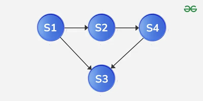
Explanation:
- Transitions are from the S1 to S2, S1 to S3, S2 to S4 and S3 to S4.
Example 5: Write state transition matrix for expression: A → B → C → D, D → B.
Solution:
State Transition Matrix = \begin{bmatrix}
0 & 1 & 0 & 0 \\
0 & 0 & 1 & 0 \\
0 & 0 & 0 & 1 \\
0.5 & 0 & 0 & 0
\end{bmatrix}
Diagram:

Explanation:
- Transitions occur in a chain from A to B to C to D with the transition from the D back to B.
Practical Questions on State Transition Matrix and Diagram
Q1: Given the states A, B, C and D with the transitions A\rightarrow B, B \rightarrow C, C \rightarrow D and D \rightarrow A construct the State Transition Matrix and Diagram.
Q2: A system has states X, Y, Z with the transitions X \rightarrow Y, Y \rightarrow Z, Z \rightarrow X . Create the State Transition Matrix and Diagram.
Q3: For a system with states P, Q, R where P \rightarrow Q , P \rightarrow R, Q \rightarrow R and R \rightarrow P determine the State Transition Matrix and Diagram.
Q4: Construct the State Transition Matrix and Diagram for a system with states A, B and C with the transitions A \rightarrow B, B \rightarrow C, C \rightarrow B and C \rightarrow A.
Q5: Given the states 1, 2, 3, 4 and transitions 1 \rightarrow 2, 2 \rightarrow 3, 3 \rightarrow 4 and 4 \rightarrow 1 find the State Transition Matrix and Diagram.
Q6: For a system with states L, M, N where L \rightarrow M, M \rightarrow N, N \rightarrow L and M \rightarrow L create the State Transition Matrix and Diagram.
Q7: Create the State Transition Matrix and Diagram for a system with states I, II, III and transitions I \rightarrow II, II \rightarrow III, III \rightarrow II and III \rightarrow I.
Q8: A system has states A, B, C, D with the transitions A \rightarrow B, B \rightarrow C, C \rightarrow D and D \rightarrow B. Construct the State Transition Matrix and Diagram.
Q9: Given states 1, 2, 3, 4 with transitions 1 \rightarrow 2, 2 \rightarrow 3, 3 \rightarrow 4 and 4 \rightarrow 1 and an additional transition 1 \rightarrow 3 find the State Transition Matrix and Diagram.
Q10: For a system with the states X, Y, Z where X \rightarrow Y, Y \rightarrow Z, Z \rightarrow X and additional transitions X \rightarrow Z create the State Transition Matrix and Diagram.
Conclusion
The State Transition Matrices and Diagrams are essential tools for the modeling and understanding complex systems that transition between the different states. They provide the clear and structured way to the analyze system behavior, predict outcomes and ensure that systems operate correctly. The Mastering these concepts is invaluable for the anyone involved in the fields that require system modeling and analysis.
Read More,