


![Preface
Nonlinearity is a frequent visitor to engineering structures which can modify—
sometimes catastrophically—the design behaviour of the systems. The best laid
plans for a linear system will often go astray due to, amongst other things,
clearances and interfacial movements in the fabricated system. There will be
situations where this introduces a threat to human life; several illustrations
spring to mind. First, an application in civil engineering. Many demountable
structures such as grandstands at concerts and sporting events are prone
to substantial structural nonlinearity as a result of looseness of joints, this
creates both clearances and friction and may invalidate any linear-model-based
simulations of the behaviour created by crowd movement. A second case comes
from aeronautical structural dynamics; there is currently major concern in the
aerospace industry regarding the possibility of limit cycle behaviour in aircraft,
i.e. large amplitude coherent nonlinear motions. The implications for fatigue
life are serious and it may be that the analysis of such motions is as important
as standard flutter clearance calculations. There are numerous examples from
the automotive industry; brake squeal is an irritating but non-life-threatening
example of an undesirable effect of nonlinearity. Many automobiles have
viscoelastic engine mounts which show marked nonlinear behaviour: dependence
on amplitude, frequency and preload. The vast majority of engineers—from all
flavours of the subject—will encounter nonlinearity at some point in their working
lives, and it is therefore desirable that they at least recognize it. It is also desirable
that they should understand the possible consequences and be in a position to take
remedial action. The object of this book is to provide a background in techniques
specific to the field of structural dynamics, although the ramifications of the theory
extend beyond the boundaries of this discipline.
Nonlinearity is also of importance for the diagnosis of faults in structures. In
many cases, the occurrence of a fault in an initially linear structure will result in
nonlinear behaviour. Another signal of the occurrence of damage is the variation
with time of the system characteristics.
The distinction between linear and nonlinear systems is important; nonlinear
systems can exhibit extremely complex behaviour which linear systems cannot.
The most spectacular examples of this occur in the literature relating to chaotic
systems [248]; a system excited with a periodic driving force can exhibit an
Copyright © 2001 IOP Publishing Ltd](https://image.slidesharecdn.com/72268096-non-linearity-in-structural-dynamics-detection-identification-and-modelling-copy-120717010202-phpapp02/85/72268096-non-linearity-in-structural-dynamics-detection-identification-and-modelling-copy-12-320.jpg)
![apparently random response. In contrast, a linear system always responds to a
periodic excitation with a periodic signal at the same frequency. At a less exotic
level, but no less important for that, the stability theory of linear systems is well
understood [207]; this is emphatically not the case for nonlinear systems.
The subject of nonlinear dynamics is extremely broad and an extensive
literature exists. This book is inevitably biased towards those areas which the
authors are most familiar with and this of course means those areas which the
authors and colleagues have conducted research in. This review is therefore as
much an expression of personal prejudice and taste as anything else, and the
authors would like to sincerely apologise for any inadvertent omissions. This is
not to say that there are no deliberate omissions; these have good reasons which
are explained here.
¯ There is no real discussion of nonlinear dynamical systems theory, i.e. phase
space analysis, bifurcations of systems and vector fields, chaos. This is a
subject best described by the more mathematically inclined and the reader
should refer to many excellent texts. Good introductions are provided by
[79] and [12]. The monograph [125] is already a classic and an overview
suited to the Engineer can be found in [248].
¯ There is no attempt to summarize many of the developments originating
in control theory. The geometrical approach to nonlinearity pioneered by
Brockett has led to very little concrete progress in mainstream structural
dynamics beyond making rigorous some of the techniques adopted lately.
The curious reader is directed to the introduction [259] or to the classic
monograph [136]. Further, there is no discussion of any of the schemes
based on Kalman filtering—again the feeling of the authors is that this is
best left to control engineers.
¯ There is no discussion of some of the recent approaches based on spectral
methods. Many of these developments can be traced back to the work
of Bendat, who has summarized the background admirably in his own
monograph [25] and the recent update [26]. The ‘reverse-path’ approach
typified by [214] can be traced back through the recent literature survey
[2]. The same authors, Adams and Allemang, have recently proposed an
interesting method based on frequency response function analysis, but it is
perhaps a little early to judge [3].
¯ There is no discussion of nonlinear normal modes. Most research in
structural dynamics in the past has concentrated on the effect of nonlinearity
on the resonant frequencies of systems. Recently, there has been interest in
estimating the effect on the modeshapes. The authors here feel that this has
been dealt with perfectly adequately in the monograph [257]. There is also a
useful recent review article [258].
So, what is in this book? The following is a brief outline.
Chapter 1 describes the relevant background in linear structural dynamics. This
is needed to understand the rest of the book. As well as describing
Copyright © 2001 IOP Publishing Ltd](https://image.slidesharecdn.com/72268096-non-linearity-in-structural-dynamics-detection-identification-and-modelling-copy-120717010202-phpapp02/85/72268096-non-linearity-in-structural-dynamics-detection-identification-and-modelling-copy-13-320.jpg)


![Chapter 1
Linear systems
This chapter is provided more or less as a reminder of linear system theory. It is
not comprehensive and it is mainly intended to set the scene for the later material
on nonlinearity. It brings to the attention of the reader the basic properties of linear
systems and establishes notation. Parts of the theory which are not commonly
covered in elementary textbooks are treated in a little more detail.
Any book on engineering dynamics or mechanical vibrations will serve as
reference for the following sections on continuous-time systems, e.g. Thompson
[249] or the more modern work by Inman [135]. For the material on discrete-time
systems, any recent book on system identification can be consulted, S¨ derstrom
o
and Stoica [231] is an excellent example.
1.1 Continuous-time models: time domain
How does one begin to model dynamical systems? Starting with the simplest
possible system seems to be sensible; it is therefore assumed that the system is
a single point particle of mass Ñ moving in one dimension subject to an applied
force ܴص1 . The equation of motion for such an object is provided by Newton’s
second law,
´ÑÚµ ܴص (1.1)
Ø
where Ú is the velocity of the particle. If the mass Ñ is constant, the equation
becomes
Ñ ´Øµ ܴص (1.2)
where ´Øµ is the acceleration of the particle. If the displacement Ý ´Øµ of
the particle is the variable of interest, this becomes a second-order differential
½ In general, the structures of Engineering significance are continuous: beams, plates, shells and
more complicated assemblies. Such systems have partial differential equations of motion dictating the
behaviour of an infinite number of degrees-of-freedom (DOF). This book is concerned only with
systems with a finite number of DOF as even a small number is sufficient to illustrate fully the
complexities of nonlinear systems.
Copyright © 2001 IOP Publishing Ltd](https://image.slidesharecdn.com/72268096-non-linearity-in-structural-dynamics-detection-identification-and-modelling-copy-120717010202-phpapp02/85/72268096-non-linearity-in-structural-dynamics-detection-identification-and-modelling-copy-17-320.jpg)

![Continuous-time models: time domain 3
The solution of (1.7) is elementary and is given in any book on vibrations or
differential equations [227]. An interesting special case is where ܴص ¼ and
one observes the unforced or free motion,
Ý· Ý ¼ (1.8)
Ñ
There is a trivial solution to this equation given by Ý ´Øµ ¼ which results
from specifying the initial conditions Ý ´¼µ ¼ and Ý´¼µ ¼. Any point at which
the mass can remain without motion for all time is termed an equilibrium or fixed
point for the system. It is clear from the equation that the only equilibrium for this
system is the origin Ý ¼, i.e. the static equilibrium position. This is typical of
linear systems but need not be the case for nonlinear systems. A more interesting
solution results from specifying the initial conditions Ý ´¼µ ,Ý ¼, i.e. the
mass is released from rest at Ø ¼ a distance from the equilibrium. In this case,
ݴص Ó×´ Ò Øµ (1.9)
Õ
This is a periodic oscillation about Ý ¼ with angular frequency Ò Ñ
Õ
½
radians per second, frequency Ò
ÔÑ ¾ Ñ Hz, and period of oscillation
ÌÒ ¾ seconds. Because the frequency is of the free oscillations it is
termed the undamped natural frequency of the system, hence the subscript Ò.
The first point to note here is that the oscillations persist without attenuation
as Ø ½. This sort of behaviour is forbidden by fundamental thermodynamic
constraints, so some modification of the model is necessary in order that free
oscillations are not allowed to continue indefinitely. If one thinks in terms of a
mass on a spring, two mechanisms become apparent by which energy is dissipated
or damped. First, unless the motion is taking place in a vacuum, there will be
resistance to motion by the ambient fluid (air in this case). Second, energy will be
dissipated in the material of the spring. Of these two dissipation processes, only
the first is understood to any great extent. Fortunately, experiment shows that it is
fairly common. In fact, at low velocities, the fluid offers a resistance proportional
to and in opposition to the velocity of the mass. The damping force is therefore
represented by ´Ý µ Ý in the model, where is the damping constant. The
equation of motion is therefore,
ÑÝ Ü´Øµ ´Ýµ Ö ´Ýµ (1.10)
or
ÑÝ · Ý · Ý Ü´Øµ (1.11)
This equation is the equation of motion of a single point mass moving in
one dimension, such a system is referred to as single degree-of-freedom (SDOF).
If the point mass were allowed to move in three dimensions, the displacement
ݴص would be a vector whose components would be specified by three equations
Copyright © 2001 IOP Publishing Ltd](https://image.slidesharecdn.com/72268096-non-linearity-in-structural-dynamics-detection-identification-and-modelling-copy-120717010202-phpapp02/85/72268096-non-linearity-in-structural-dynamics-detection-identification-and-modelling-copy-19-320.jpg)

![Continuous-time models: time domain 5
y(t)
ζωnt
Ae
t
Figure 1.2. Transient motion of a SDOF oscillator with positive damping. The envelope
of the response is also shown.
¯ If ½, the system is said to be overdamped and the situation is similar
to critical damping, the system is non-oscillatory but gradually returns to its
equilibrium when disturbed. Newland [198] gives an interesting discussion
of overdamped systems.
Consideration of the free motion has proved useful in that it has allowed
a physical positivity constraint on or to be derived. However, the most
interesting and more generally applicable solutions of the equation will be for
forced motion. If attention is restricted to deterministic force signals ܴص 2 ,
Fourier analysis allows one to express an arbitrary periodic signal as a linear
sum of sinusoids of different frequencies. One can then invoke the principle of
superposition which allows one to concentrate on the solution where ܴص is a
single sinusoid, i.e.
ÑÝ · Ý · Ý Ó×´ ص (1.15)
where ¼ and is the constant frequency of excitation. Standard differential
equation theory [227] asserts that the general solution of (1.15) is given by
ݴص ÝØ ´Øµ · Ý× ´Øµ (1.16)
where the complementary function (or transient response according to the earlier
notation) ÝØ ´Øµ is the unique solution for the free equation of motion and contains
arbitrary constants which are fixed by initial conditions. Ý Ø ´Øµ for equation (1.15)
¾ It is assumed that the reader is familiar with the distinction between deterministic signals and those
which are random or stochastic. If not, [249] is a good source of reference.
Copyright © 2001 IOP Publishing Ltd](https://image.slidesharecdn.com/72268096-non-linearity-in-structural-dynamics-detection-identification-and-modelling-copy-120717010202-phpapp02/85/72268096-non-linearity-in-structural-dynamics-detection-identification-and-modelling-copy-21-320.jpg)


![10 Linear systems
Bode plot of an actual SDOF system,
Ý · ¾¼Ý · ½¼ Ý Ü´Øµ (1.30)
(The particular routine used to generate this plot actually shows in keeping
with the conventions of [87].) For this system, the undamped natural frequency
is 100 rad s ½ , the damped natural frequency is 99.5 rad s ½ , the resonance
frequency is 99.0 rad s ½ and the damping ratio is 0.1 or 10% of critical.
A more direct construction of the system representation in terms of the Bode
plot will be given in the following section. Note that the gain and phase in
expressions (1.23) and (1.24) are independent of the magnitude of the forcing
level . This means that the FRF is an invariant of the amplitude of excitation. In
fact, this is only true for linear systems and breakdown in the amplitude invariance
of the FRF can be used as a test for nonlinearity as discussed in chapter 2.
1.2 Continuous-time models: frequency domain
The input and output time signals ܴص and Ý ´Øµ for the SDOF system discussed
earlier are well known to have dual frequency-domain representations ´ µ
ܴص and ´ µ ݴص obtained by Fourier transformation where
·½
´ µ ´Øµ Ø Ø ´Øµ (1.31)
½
3
defines the Fourier transform . The corresponding inverse transform is given
by
½ ½ ·½ Ø ´ µ
´Øµ ´ µ (1.32)
¾ ½
It is natural to ask now if there is a frequency-domain representation of the
system itself which maps ´ µ directly to ´ µ. The answer to this is yes and
the mapping is remarkably simple. Suppose the evolution in time of the signals is
specified by equation (1.11); one can take the Fourier transform of both sides of
¿ Throughout this book, the preferred notation for integrals will be
Ü ´Üµ
rather than
´Üµ Ü
This can be regarded simply as a matter of grammar. The first integral is the integral with respect to
Ü of ´Üµ, while the second is the integral of ´Üµ with respect to Ü. The meaning is the same in either
case; however, the authors feel that the former expression has more formal significance in keeping the
integral sign and measure together. It is also arguable that the notation adopted here simplifies some
of the manipulations of multiple integrals which will be encountered in later chapters.
Copyright © 2001 IOP Publishing Ltd](https://image.slidesharecdn.com/72268096-non-linearity-in-structural-dynamics-detection-identification-and-modelling-copy-120717010202-phpapp02/85/72268096-non-linearity-in-structural-dynamics-detection-identification-and-modelling-copy-26-320.jpg)


![Impulse response 15
x(t)
ε ε t
Figure 1.11. Example of a transient excitation whose duration is ¾ .
where the function ´Øµ is the inverse Fourier transform of À ´ µ. If one repeats
this argument but takes the inverse transform of À ´ µ before ´ µ one obtains
the alternative expression
·½
ݴص ´ µÜ´Ø µ (1.45)
½
These equations provide another time-domain version of the system’s input–
output relationship. All system information is encoded in the function ´Øµ. One
can now ask if ´Øµ has a physical interpretation. Again the answer is yes, and the
argument proceeds as follows.
Suppose one wishes to know the response of a system to a transient input, i.e.
ܴص where ܴص ¼ if Ø ¯ say (figure 1.11). All the energy is communicated
to the system in time ¾¯ after which the system follows the unforced equations of
motion. An ideal transient excitation or impulse would communicate all energy in
an instant. No such physical signal exists for obvious reasons. However, there is
a mathematical object, the Dirac Æ -function Æ ´Øµ [166], which has the properties
of an ideal impulse:
infinitesimal duration
ƴص ¼ Ø ¼ (1.46)
finite power
·½
Ø Ü´Øµ ¾ ½ (1.47)
½
The defining relationship for the Æ -function is [166]
·½
Ø ´ØµÆ´Ø µ ´ µ for any ´Øµ (1.48)
½
Copyright © 2001 IOP Publishing Ltd](https://image.slidesharecdn.com/72268096-non-linearity-in-structural-dynamics-detection-identification-and-modelling-copy-120717010202-phpapp02/85/72268096-non-linearity-in-structural-dynamics-detection-identification-and-modelling-copy-31-320.jpg)

![Discrete-time models: time domain 17
more rigorous approach to evaluating ´Øµ is simple to formulate but complicated
by the need to use the calculus of residues.
According to the definition,
½ À ´ µ ½ ·½ Ø
´Øµ ¾ ¾·¾
¾ Ñ ½ Ò Ò
·½ Ø
¾ ½Ñ ´ · µ´ (1.55)
½ µ
where ¦ Ò¦ so that · ¾ . Partial fraction expansion of
the last expression gives
½ ·½ Ø ·½ Ø
´Øµ
Ñ ½ ´ µ ½ ´ ·µ (1.56)
The two integrals can be evaluated by contour integration [234],
·½ Ø
¾ ¦ Ø ¢´Øµ
½ ´ ¦µ
(1.57)
where ¢´Øµ is the Heaviside function defined by ¢´Øµ ½, Ø ¼, ¢´Øµ ¼,
Ø ¼, substituting into the last expression for the impulse response gives
´Øµ ´ Ø · Ø µ¢´Øµ (1.58)
¾Ñ
and substituting for the values of ¦ yields the final result, in agreement with
(1.54),
½ Ø × Ò´
´Øµ Ò Øµ¢´Øµ (1.59)
Ñ
Finally, a result which will prove useful later. Suppose that one excites a
system with a signal Ø (clearly this is physically unrealizable as it is complex),
the response is obtained straightforwardly from equation (1.45),
·½
ݴص ´ µ ´Ø µ (1.60)
½
·½
Ø ´ µ À´ µ Ø (1.61)
½
so the system response to the input Ø is À ´ µ Ø. One can regard this result
as giving an alternative definition of the FRF.
1.4 Discrete-time models: time domain
The fact that Newton’s laws of motion are differential equations leads directly
to the continuous-time representation of previously described systems. This
Copyright © 2001 IOP Publishing Ltd](https://image.slidesharecdn.com/72268096-non-linearity-in-structural-dynamics-detection-identification-and-modelling-copy-120717010202-phpapp02/85/72268096-non-linearity-in-structural-dynamics-detection-identification-and-modelling-copy-33-320.jpg)

![Discrete-time models: time domain 19
Ü together with values for Ý ½ and ݾ . The specification of the first two values
of the output sequence is directly equivalent to the specification of initial values
for Ý ´Øµ and Ý ´Øµ in the continuous-time case. An obvious advantage of using
a discrete model like (1.67) is that it is much simpler to numerically predict the
output in comparison with a differential equation. The price one pays is a loss
of generality—because the coefficients in (1.67) are functions of the sampling
interval ¡Ø, one can only use this model to predict responses with the same
spacing in time.
Although arguably less familiar, the theory for the solution of difference
equations is no more difficult than the corresponding theory for differential
equations. A readable introduction to the relevant techniques is given in
chapter 26 of [233].
Consider the free motion for the system in (1.67); this is specified by
Ý ½ Ý ½ · ¾ Ý ¾ (1.68)
Substituting a trial solution Ý « with « constant yields
« ¾ ´«¾ ½ « ¾ µ ¼ (1.69)
which has non-trivial solutions
Õ
½¦½
«¦
¾ ¾ ¾· ¾
½ (1.70)
The general solution of (1.68) is, therefore,
Ý «· · « (1.71)
where and are arbitrary constants which can be fixed in terms of the initial
values ݽ and ݾ as follows. According to the previous solution Ý ½ «· · «
and ݾ «¾ · «¾ ; these can be regarded as simultaneous equations for
·
and , the solution being
ݾ « ݽ
«· ´«· « µ
(1.72)
«· ݽ ݾ
« ´«· « µ
(1.73)
Analysis of the stability of this system is straightforward. If either « · ½
or « ½ the solution grows exponentially, otherwise the solution decays
exponentially. More precisely, if the magnitudes of the ÐÔ s are greater than
one—as they may be complex—the solutions are unstable. In the differential
equation case the stability condition was simply ¼. The stability condition
in terms of the difference equation parameters is the slightly more complicated
expression ¬ ¬
Õ
¬ ½¦½ ¬
¬
¬ ¾ ¾ ¾ · ¾¬ ½
½¬ (1.74)
Copyright © 2001 IOP Publishing Ltd](https://image.slidesharecdn.com/72268096-non-linearity-in-structural-dynamics-detection-identification-and-modelling-copy-120717010202-phpapp02/85/72268096-non-linearity-in-structural-dynamics-detection-identification-and-modelling-copy-35-320.jpg)

![Classification of difference equations 21
One point about these equations is worth noting. The expressions for gain and
phase are functions of frequency through the variables and Ë . However,
½
these variables are periodic with period ¡Ø × . As a consequence, the gain and
phase formulae simply repeat indefinitely as ½. This means that knowledge
of the response functions in the interval ¾× ¾× is sufficient to specify them for
all frequencies. An important consequence of this is that a discrete representation
of a system can be accurate in the frequency domain only on a finite interval. The
frequency ¾× which prescribes this interval is called the Nyquist frequency.
1.5 Classification of difference equations
Before moving on to consider the frequency-domain representation for discrete-
time models it will be useful to digress slightly in order to discuss the taxonomy
of difference equations, particularly as they will feature in later chapters. The
techniques and terminology of discrete modelling has evolved over many years
in the literature of time-series analysis, much of which may be unfamiliar to
engineers seeking to apply these techniques. The aim of this section is simply
to describe the basic linear difference equation structures, the classic reference
for this material is the work by Box and Jenkins [46].
1.5.1 Auto-regressive (AR) models
As suggested by the name, an auto-regressive model expresses the present output
Ý from a system as a linear combination of past outputs, i.e. the variable is
regressed on itself. The general expression for such a model is
Ô
Ý Ý (1.83)
½
and this is termed an AR(Ô) model.
1.5.2 Moving-average (MA) models
In this case the output is expressed as a linear combination of past inputs. One
can think of the output as a weighted average of the inputs over a finite window
which moves with time, hence the name. The general form is
Õ
Ý Ü (1.84)
½
and this is called a MA(Õ ) model.
All linear continuous-time systems have a canonical representation as a
moving-average model as a consequence of the input–output relationship:
·½
Ý ´Ø µ ´ µÜ´Ø µ (1.85)
¼
Copyright © 2001 IOP Publishing Ltd](https://image.slidesharecdn.com/72268096-non-linearity-in-structural-dynamics-detection-identification-and-modelling-copy-120717010202-phpapp02/85/72268096-non-linearity-in-structural-dynamics-detection-identification-and-modelling-copy-37-320.jpg)

![Multi-degree-of-freedom (MDOF) systems 23
Now one defines the FRF À ´ µ by the means suggested at the end of
section 1.3. If the input to the system is Ø , the output is À ´ µ Ø . The action
of on the signals is given by
ÑÜ Ñ ¡Ø ´ ѵ¡Ø Ñ ¡ØÜ (1.91)
on the input and
ÑÝ Ñ À´ µÜ À ´ µ Ñ ¡Ø
À ´ µ ´ ѵ¡Ø À ´ µ Ñ ¡ØÜ (1.92)
on the output. Substituting these results into equation (1.90) yields
Ô Õ
½ ¡Ø À ´ µÜ ¡Ø Ü (1.93)
½ ½
which, on simple rearrangement, gives the required result
ÈÕ ¡Ø
À´ µ ½
ÈÔ
´½ ½ ¡Ø µ (1.94)
Note that this expression is periodic in as discussed at the close of
section 1.4.
1.7 Multi-degree-of-freedom (MDOF) systems
The discussion so far has been restricted to the case of a single mass point. This
has proved useful in that it has allowed the development of most of the basic
theory used in modelling systems. However, the assumption of single degree-of-
freedom behaviour for all systems is clearly unrealistic. In general, one will have
to account for the motion of several mass points or even a continuum. To see this,
consider the transverse vibrations of a simply supported beam (figure 1.12). A
basic analysis of the statics of the situation, shows that an applied force at the
centre of the beam produces a displacement Ý given by
Á
Ý
Ä¿
(1.95)
where is the Young’s modulus of the beam material, Á is the second moment of
area and Ä is the length of the beam. is called the flexural stiffness.
If it is now assumed that the mass is concentrated at the centre (figure 1.13),
by considering the kinetic energy of the beam vibrating with a maximum
displacement at the centre, it can be shown that the point mass is equal to half
the total mass of the beam Å ¾ [249]. The appropriate equation of motion is
Å
· Ý Ü´Øµ (1.96)
¾
Copyright © 2001 IOP Publishing Ltd](https://image.slidesharecdn.com/72268096-non-linearity-in-structural-dynamics-detection-identification-and-modelling-copy-120717010202-phpapp02/85/72268096-non-linearity-in-structural-dynamics-detection-identification-and-modelling-copy-39-320.jpg)


![34 Linear systems
and from (1.139) it follows that
Ì ¼ (1.143)
So the modeshapes belonging to distinct eigenvalues are orthogonal with
respect to the mass and stiffness matrices. This is referred to as weighted
orthogonality. The situation where the eigenvalues are not distinct is a little
more complicated and will not be discussed here, the reader can refer to [87].
Note that unless the mass or stiffness matrix is the unit, the eigenvectors or
modeshapes are not orthogonal in the usual sense, i.e. Ì ¼. Assuming
Ò distinct eigenvalues, one can form the modal matrix © by taking an array of
the modeshapes
© ½ ¾ Ò (1.144)
Consider the matrix
Å ©ÌÑ © (1.145)
A little algebra shows that the elements are
Å ÌÑ (1.146)
and these are zero if by the weighted orthogonality (1.142). This means
that Å is diagonal. The diagonal elements Ñ ½ Ѿ ÑÒ are referred to as
the generalized masses or modal masses as discussed in the previous section. By
a similar argument, the matrix
à ©Ì © (1.147)
is diagonal with elements ½ ¾ Ò which are termed the generalized or
modal stiffnesses. The implications for the equations of motion (1.133) are
important. Consider the change of coordinates
© Ù Ý (1.148)
equation (1.133) becomes
Ñ © Ù · © Ù ¼ (1.149)
and premultiplying by © Ì gives
©ÌÑ © Ù · ©Ì © Ù ¼ (1.150)
or
Å Ù ·Ã Ù ¼ (1.151)
by virtue of equations (1.145) and (1.147). The system has been decoupled into
Ò SDOF equations of motion of the form
ÑÙ · Ù ¼ ½ Ò (1.152)
Copyright © 2001 IOP Publishing Ltd](https://image.slidesharecdn.com/72268096-non-linearity-in-structural-dynamics-detection-identification-and-modelling-copy-120717010202-phpapp02/85/72268096-non-linearity-in-structural-dynamics-detection-identification-and-modelling-copy-50-320.jpg)

![36 Linear systems
with termed the (viscous) damping matrix. (In many cases, it will be desirable
to consider structural damping, the reader is referred to [87].) The desired result
is to decouple the equations (1.160) into SDOF oscillators in much the same way
as for the damped case. Unfortunately, this is generally impossible as observed
in the last section. While it is (almost) always possible to find a matrix © which
diagonalizes two matrices ( Ñ and ), this is not the case for three ( Ñ , and
). Rather than give up, the usual recourse is to assume Rayleigh or proportional
damping as in (1.114) 8. In this case,
©Ì © ´½ Òµ (1.162)
with
«Ñ · ¬ (1.163)
With this assumption, the modal matrix decouples the system (1.160) into
Ò SDOF systems in much the same way as for the undamped case, the relevant
equations are (after the transformation (1.148)),
ÑÙ · Ù · Ù ¼ ½ Ò (1.164)
and these have solutions
Ù Ò Ø × Ò´ Ø µ (1.165)
where and are fixed by the initial conditions and
¾ Ñ
Ô (1.166)
is the th modal damping ratio and
¾ ¾ ´½ ¾ µ
Ò (1.167)
is the th damped natural frequency. Transforming back to physical coordinates
using (1.148) yields
Ò
Ý © Ò Ø × Ò´ Ø µ (1.168)
½
One can do slightly better than traditional proportional damping. It is known that if a matrix ©
diagonalizes Ñ , then it also diagonalizes ´ µ
Ñ where is a restricted class of matrix functions.
( must have a Laurent expansion of the form
´Ñµ ½ Ñ ½ · ¼ ½
· ½ Ñ · ¾Ñ¾
functions like Ø Ñ are not allowed for obvious reasons.) Similarly, if © diagonalizes , it will
also diagonalize ´ µ if belongs to the same class as . In principle, one can choose any damping
matrix
´Ñµ· ´Ñµ
and will diagonalize it, i.e.
©Ì © ´ ´Ñ½ µ · ´ ½ µ ´ÑÒ µ · ´ Ò µµ
Having said this, this freedom is never used and the most common choice of damping prescription
is proportional.
Copyright © 2001 IOP Publishing Ltd](https://image.slidesharecdn.com/72268096-non-linearity-in-structural-dynamics-detection-identification-and-modelling-copy-120717010202-phpapp02/85/72268096-non-linearity-in-structural-dynamics-detection-identification-and-modelling-copy-52-320.jpg)

![38 Linear systems
In terms of the individual elements of À , (1.177) yields
Ò Ò Ò
À ´ µ Ð ´ µÐ Ì ´ µ (1.178)
Ð ½ ½ ½
and finally
Ò
À ´ µ ¾·
½ Ñ
(1.179)
·
or
Ò
À ´ µ ¾
¾ Ò µ·¾
½ ´
(1.180)
Ò
where
(1.181)
Ñ
are the residues or modal constants.
It follows from these equations that the FRF for any process Ü Ý of a
MDOF linear system is the sum of Ò SDOF FRFs, one for each natural frequency.
It is straightforward to show that each individual mode has a resonant frequency,
Õ
Ö Ò ½ ¾ ¾ (1.182)
Taking the inverse Fourier transform of the expression (1.180) gives the
general form of the impulse response for a MDOF system
Ò
´Øµ Ø Ó×´ Ø µ (1.183)
½
and the response of a general MDOF system to a transient is a sum of decaying
harmonics with individual decay rates and frequencies.
A final remark is required about the proportionality assumption for the
damping. For a little more effort than that expended here, one can obtain the
system FRFs for an arbitrarily damped linear system [87]. The only change in the
final form (1.181) is that the constants become complex.
All these expressions are given in receptance form; parallel mobility and
accelerance forms exist and are obtained by multiplying the receptance form by
and ¾ respectively.
There are well-established signal-processing techniques which allow one to
experimentally determine the FRFs of a system. It is found for linear structural
systems that the representation as a sum of resonances given in (1.181) is
remarkably accurate. An example of a MDOF FRF is given in figure 1.20. After
obtaining an experimental curve for some À ´ µ the data can be curve-fitted to
the form in equation (1.181) and the best-fit values for the parameters Ñ ,
Copyright © 2001 IOP Publishing Ltd](https://image.slidesharecdn.com/72268096-non-linearity-in-structural-dynamics-detection-identification-and-modelling-copy-120717010202-phpapp02/85/72268096-non-linearity-in-structural-dynamics-detection-identification-and-modelling-copy-54-320.jpg)


![Symptoms of nonlinearity 49
2.2.3 Homogeneity and FRF distortion
This represents a restricted form of the principle of superposition. It is
undoubtedly the most common method in use for detecting the presence of
nonlinearity in dynamic testing. Homogeneity is said to hold if ܴص Ý ´Øµ
implies «Ü´Øµ «Ý ´Øµ for all «. In essence, homogeneity is an indicator of
the system’s insensitivity to the magnitude of the input signal. For example, if
an input «Ü½ ´Øµ always produces an output «Ý ½ ´Øµ, the ratio of output to input is
independent of the constant «. The most striking consequence of this is in the
frequency domain. First, note that «Ü´Øµ «Ý ´Øµ implies « ´ µ « ´ µ.
This means that if ܴص «Ü´Øµ,
´ µ « ´ µ
À´ µ
´ µ
« ´ µ
À´ µ (2.21)
and the FRF is invariant under changes of « or effectively of the level of
excitation.
Because of this, the homogeneity test is usually applied in dynamic testing
to FRFs where the input levels are usually mapped over a range encompassing
typical operating levels. If the FRFs for different levels overlay, linearity is
assumed to hold. This is not infallible as there are some systems which are
nonlinear which nonetheless show homogeneity; the bilinear system discussed
in the next chapter is an example. The reason for this is that homogeneity is a
weaker condition than superposition.
An example of the application of a homogeneity test is shown in figure 2.7.
In this case band-limited random excitation has been used but, in principle, any
type of excitation signal may be employed. Although a visual check is often
sufficient to see if there are significant differences between FRFs, other metrics
can be used such as a measure of the mean-square error between the FRFs. The
exact form of the distortion in the FRF depends on the type of the nonlinearity,
some common types of FRF distortion produced by varying the level of excitation
are discussed in the following section.
One possible problem with the homogeneity test is caused by force ‘drop-
out’. Drop-out is a common phenomenon which occurs when forced vibration
tests are carried out during dynamic testing. As its description implies, this is
a reduction in the magnitude of the input force spectrum measured by the force
transducer and occurs in the vicinity of the resonant frequencies of the structure
under test. It is a result of the interaction between an electrodynamic exciter and
the structure [251]. A typical experimental force drop-out characteristic is shown
in figure 2.8.
If homogeneity is being used as a detection method for nonlinearity, force
drop-out can create misleading results. This is because the test for homogeneity
assumes that the input is persistently exciting, i.e. exercises the system equally
across the whole excitation bandwidth, whereas the effect of force drop-out is to
effectively notch-filter the input at the resonant frequency. This results in less
Copyright © 2001 IOP Publishing Ltd](https://image.slidesharecdn.com/72268096-non-linearity-in-structural-dynamics-detection-identification-and-modelling-copy-120717010202-phpapp02/85/72268096-non-linearity-in-structural-dynamics-detection-identification-and-modelling-copy-65-320.jpg)


![Common types of nonlinearity 53
Force
Force
Force
Displacement Displacement Displacement
Hardening Softening
Cubic Stiffness Bilinear Stiffness
Force
Force
Displacement Displacement
Saturation (or limiter) Clearance (or backlash)
Force
Force
Velocity Velocity
Coulomb Friction Nonlinear Damping
Figure 2.10. Idealized forms of simple structural nonlinearities.
The equation of motion of the SDOF oscillator with linear damping and
stiffness (2.23) is called Duffing’s equation [80],
ÑÝ · Ý · Ý · ¿ Ý ¿ ܴص (2.24)
and this is the single most-studied equation in nonlinear science and engineering.
The reason for its ubiquity is that it is the simplest nonlinear oscillator which
possesses the odd symmetry which is characteristic of many physical systems.
Despite its simple structure, it is capable of showing almost all of the interesting
behaviours characteristic of general nonlinear systems. This equation will re-
occur many times in the following chapters.
The FRF distortion characteristic of these systems is shown in figures 2.11(b)
and (c). The most important point is that the resonant frequency shifts up for the
hardening system as the level of excitation is raised, this is consistent with the
Copyright © 2001 IOP Publishing Ltd](https://image.slidesharecdn.com/72268096-non-linearity-in-structural-dynamics-detection-identification-and-modelling-copy-120717010202-phpapp02/85/72268096-non-linearity-in-structural-dynamics-detection-identification-and-modelling-copy-69-320.jpg)

![Common types of nonlinearity 55
increase in effective stiffness. As one might expect, the resonant frequency for
the softening system shifts down.
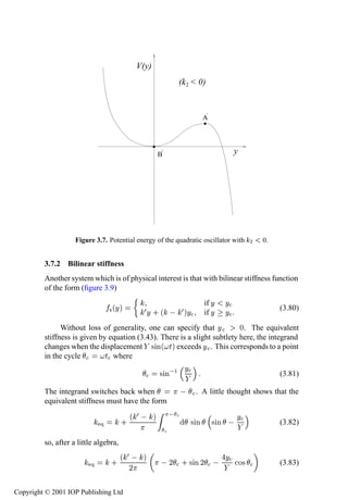
2.3.2 Bilinear stiffness or damping
In this case, the stiffness characteristic has the form,
× ´Ýµ ½Ý Ý ¼ (2.25)
¾Ý Ý ¼
with a similar definition for bilinear damping. The most extreme example of a
bilinear system is the impact oscillator for which ½ ¼ and ¾ ½; this
corresponds to a ball bouncing against a hard wall. Such systems can display
extremely complex behaviour indeed (see chapter 15 of [248]). One system
which approximates to a bilinear damping system is the standard automotive
damper or shock absorber which is designed to have different damping constants
in compression and rebound. Such systems are discussed in detail in chapters 7
and 9.
Figure 2.11 does not show the FRF distortion characteristic of this system
because it is one of the rare nonlinear systems which display homogeneity. (This
last remark is only true if the position of the change in stiffness is at the origin, if
it is offset by any degree, the system will fail to show homogeneity if the level of
excitation is taken sufficiently high.)
2.3.3 Piecewise linear stiffness
The form of the stiffness function in this case is
¾Ý · ´ ½ ¾µ Ý
× ´Ýµ ½Ý Ý (2.26)
¾Ý ´ ½ ¾µ Ý .
Two of the nonlinearities in figure 2.10 are special cases of this form. The
saturation or limiter nonlinearity has ¾ ¼ and the clearance or backlash
nonlinearity has ½ ¼.
In aircraft ground vibration tests, nonlinearities of this type can arise from
assemblies such as pylon–store–wing assemblies or pre-loading bearing locations.
Figure 2.12 shows typical results from tests on an aircraft tail-fin where the
resonant frequency of the first two modes reduces as the input force level is
increased and then asymptotes to a constant value. Such results are typical of
pre-loaded backlash or clearance nonlinearities.
Typical FRF distortion is shown in figure 2.11(f ) for a hardening piecewise
linear characteristic ( ¾ ½ ).
Copyright © 2001 IOP Publishing Ltd](https://image.slidesharecdn.com/72268096-non-linearity-in-structural-dynamics-detection-identification-and-modelling-copy-120717010202-phpapp02/85/72268096-non-linearity-in-structural-dynamics-detection-identification-and-modelling-copy-71-320.jpg)
![56 From linear to nonlinear
21
.
6
Response Amplitude (g)
..
5
.. Frequency
Frequency (Hz)
.
.
20
4
.
Accel 04
.
.
3
.
Amplitude
19
2
..
. . .. .
. ..
1
18
0
0 6 12 18 24 30 36
Input Force (N)
79
8
.
Response Amplitude (g)
Frequency (Hz)
.
6
Frequency
Accel 00
.
78
.
4
.
. . Amplitude
. .
2
. .
.
77
0
0 5 10 15 20 25
Input Force (N)
Figure 2.12. Results from ground vibration tests on the tail-fin of an aircraft showing
significant variation in the resonant frequency with increasing excitation level. This was
traced to clearances in the mounting brackets.
2.3.4 Nonlinear damping
The most common form of polynomial damping is quadratic:
´Ýµ ¾Ý Ý (2.27)
(where the absolute value term is to ensure that the force is always opposed to
the velocity). This type of damping occurs when fluid flows through an orifice or
around a slender member. The former situation is common in automotive dampers
and hydromounts, the latter occurs in the fluid loading of offshore structures. The
fundamental equation of fluid loading is Morison’s equation [192],
´Øµ
½ ٴص · ¾ ٴص ٴص (2.28)
where is the force on the member and Ù is the velocity of the flow. This system
will be considered in some detail in later chapters.
Copyright © 2001 IOP Publishing Ltd](https://image.slidesharecdn.com/72268096-non-linearity-in-structural-dynamics-detection-identification-and-modelling-copy-120717010202-phpapp02/85/72268096-non-linearity-in-structural-dynamics-detection-identification-and-modelling-copy-72-320.jpg)

![58 From linear to nonlinear
measurement of FRFs or spectra it is strongly recommended that a visual check
is maintained of the individual drive/excitation and response voltage signals. This
can be done very simply by the use of an oscilloscope.
In modal testing it is usual to use a force transducer (or transducers in
the case of multi-point testing) as the reference input signal. Under such
circumstances it is strongly recommended that this signal is continuously (or at
least periodically) monitored on an oscilloscope. This is particularly important
as harmonic distortion of the force excitation signal is not uncommon, often due
to shaker misalignment or ‘force drop-out’ at resonance. Distortion can create
errors in the measured FRF which may not be immediately apparent and it is very
important to ensure that the force input signal is not distorted.
Usually in dynamic testing one may have the choice of observing the
waveform in terms of displacement, velocity or acceleration. For a linear system
in which no distortion of the signal occurs it makes little difference which variable
is used. However, when nonlinearity is present this generally results in harmonic
distortion. As discussed earlier in this chapter, under sinusoidal excitation,
harmonic distortion is much easier to observe when acceleration is measured.
Thus it is recommended that during testing with a sine wave, a simple test of the
quality of the output waveform is to observe it on an oscilloscope in terms of the
acceleration response. Any distortion or noise present will be more easily visible.
Due to their nature, waveform distortion in random signals is more difficult
to observe using an oscilloscope than with a sine-wave input. However, it is still
recommended that such signals are observed on an oscilloscope during testing
since the effect of extreme nonlinearities such as clipping of the waveforms can
easily be seen.
The first two problems previously itemized will be discussed in a little more
detail.
2.4.1 Misalignment
This problem often occurs when electrodynamic exciters are used to excite
structures in modal testing. If an exciter is connected directly to a structure
then the motion of the structure can impose bending moments and side loads
on the exciter armature and coil assembly resulting in misalignment, i.e. the coil
rubbing against the internal magnet of the exciter. Misalignment can be detected
by using a force transducer between the exciter and the test structure, the output
of which should be observed on an oscilloscope. If a sine wave is injected into
the structure, misalignment will produce a distorted force signal which, if severe,
may appear as shown in figure 2.6. If neglected, this can create significant damage
to the vibration exciter coil, resulting in a reduction in the quality of the FRFs and
eventual failure of the exciter. To minimize this effect it is recommended that a
‘stinger’ or ‘drive-rod’ is used between the exciter and the test structure described
in [87].
Copyright © 2001 IOP Publishing Ltd](https://image.slidesharecdn.com/72268096-non-linearity-in-structural-dynamics-detection-identification-and-modelling-copy-120717010202-phpapp02/85/72268096-non-linearity-in-structural-dynamics-detection-identification-and-modelling-copy-74-320.jpg)


![68 From linear to nonlinear
by dividing the Fourier transform of the response by the Fourier transform of the
force. Averaging is usually carried out and this means that a coherence function
can be estimated. The pulse used here was selected so that the maximum value
of the response in the time domain was similar to the resonant amplitude from
the sine-wave test of the last section. The results in figure 2.17(b) confirm the
earlier remarks in that a completely different FRF is obtained to that using sine
excitation.
2.6.3 Chirp excitation
A second form of transient excitation commonly used for measuring FRFs is chirp
excitation. This form of excitation can be effective in detecting nonlinearity and
combines the attraction of being relatively fast with an equal level of input power
across a defined frequency range. Chirp excitation can be linear or nonlinear
where the nonlinear chirp signal can be designed to have a specific input power
spectrum that can vary within a given frequency range [265]. The simplest form
of chirp has a linear sweep characteristic so the signal takes the form
ܴص × Ò´«Ø · ¬Ø¾ µ (2.52)
where « and ¬ are chosen to give appropriate start and end frequencies. At any
given time, the instantaneous frequency of the signal is
´Øµ ´«Ø · ¬Ø¾ µ « · ¾¬Ø (2.53)
Ø
As one might imagine, the response of a nonlinear system to such
a comparatively complex input may be quite complicated. The FRF in
figure 2.17(c) was obtained using a force consisting of a frequency sweep between
0 and 2 Hz in 50 s. (This sweep is rapid compared with the decay time of the
structure.) The FRF was once again determined from the ratio of the Fourier
transforms. The excitation level was selected so that the maximum displacement
in the time-domain was the same as before. The ‘split’ response in figure 2.17(c)
is due to the presence of the nonlinearity.
2.6.4 Random excitation
The FRF of a nonlinear structure obtained from random (usually band-limited)
excitation often appears undistorted due to the randomness of the amplitude and
phase of the excitation signal creating a ‘linearized’ or ‘averaged’ FRF.
Due to this linearization, the only way in which random excitation can assist
in detecting nonlinearity is for several tests to be carried out at different rms
levels of the input excitation (auto-spectrum of the input) and the resulting FRFs
overlaid to test for homogeneity. A word of warning here. Since the total power
in the input spectrum is spread over the band-limited frequency range used, the
ability to excite nonlinearities is significantly reduced compared with sinusoidal
Copyright © 2001 IOP Publishing Ltd](https://image.slidesharecdn.com/72268096-non-linearity-in-structural-dynamics-detection-identification-and-modelling-copy-120717010202-phpapp02/85/72268096-non-linearity-in-structural-dynamics-detection-identification-and-modelling-copy-84-320.jpg)


![FRF estimators 71
Multiplying (2.55) by and averaging yields
ËÜÝ ´ µ À ´ µËÙÙ ´ µ (2.61)
and taking the ratio of (2.60) and (2.61) gives
ËÝÝ ´ µ Ë ´ µ
À ´ µ ½ · ÑÑ (2.62)
ËÜÝ ´ µ ËÙÙ ´ µ
and this means that the estimator Ë ÝÝ ËÜÝ —denoted by À ¾ ´ µ—is only equal to
À ´ µ if there is no noise on the output (Ë ÑÑ ¼). Also, as ËÑÑ ËÙÙ ¼,
the estimator is always an overestimate, i.e. À ¾ ´ µ À ´ µ if output noise is
present. The estimator is insensitive to noise on the input.
So if there is noise on the input only, one should always use À ¾ : if there is
noise only on the output, one should use À ½ . If there is noise on both signals a
compromise is clearly needed. In fact, as À ½ is an underestimate and À ¾ is an
overestimate, the sensible estimator would be somewhere in between. As one can
always interpolate between two numbers by taking the mean, a new estimator À ¿
can be defined by taking the geometric mean of À ½ and À¾ ,
×
Ô ËÑÑ ´ µ · ËÙÙ ´ µ
À¿ ´ µ À½ ´ µÀ¾ ´ µ À´ µ (2.63)
ËÒÒ ´ µ · ËÙÙ ´ µ
and this is the estimator of choice if both input and output are corrupted.
Note that a byproduct of this analysis is a general expression for the
coherence,
ËÝÜ ´ µ ¾ ½
¾´ µ ËÑÑ ´ µ ´µ (2.64)
ËÝÝ ´ µËÜÜ ´ µ ½· ½ · ËÒÒ´ µ
ËÚÚ ´ µ ËÚÚ
from which it follows that ¾ ½ if either input or output noise is present. It also
follows from (2.64), (2.62) and (2.59) that ¾ À½ À¾ or
À½ ´ µ
À¾ ´ µ
¾´ µ
(2.65)
so the three quantities are not independent.
As the effect of nonlinearity on the FRF is different to that of input noise or
output noise acting alone, one might suspect that À ¿ is the best estimator for use
with nonlinear systems. In fact it is shown in [232] that À ¿ is the best estimator
for nonlinear systems in the sense that, of the three estimators, given an input
density ËÜÜ , À¿ gives the best estimate of Ë ÝÝ via ËÝÝ À ¾ ËÜÜ . This is
a useful property if the object of estimating the FRF is to produce an effective
linearized model by curve-fitting.
Copyright © 2001 IOP Publishing Ltd](https://image.slidesharecdn.com/72268096-non-linearity-in-structural-dynamics-detection-identification-and-modelling-copy-120717010202-phpapp02/85/72268096-non-linearity-in-structural-dynamics-detection-identification-and-modelling-copy-87-320.jpg)
![72 From linear to nonlinear
2.8 Equivalent linearization
As observed in the last chapter, modal analysis is an extremely powerful theory of
linear systems. It is so effective in that restricted area that one might be tempted
to apply the procedures of modal analysis directly to nonlinear systems without
modification. In this situation, the curve-fitting algorithms used will associate a
linear system with each FRF—in some sense the linear system which explains it
best. In the case of a SDOF system, one might find the equivalent linear FRF
½
À Õ´ µ
Ñ Õ ¾ · Õ · Õ
(2.66)
which approximates most closely that of the nonlinear system. In the time domain
this implies a best linear model of the form
Ñ ÕÝ · Õ Ý · Õ Ý Ü´Øµ (2.67)
and such a model is called a linearization. As the nonlinear system FRF will
usually change its shape as the level of excitation is changed, any linearization
is only valid for a given excitation level. Also, because the form of the FRF is
a function of the type of excitation as discussed in section 2.6, different forcing
types of nominally the same amplitude will require different linearizations. These
are clear limitations.
In the next chapter, linearizations based on FRFs from harmonic forcing
will be derived. In this section, linearizations based on random excitation will
be discussed. These are arguably more fundamental because, as discussed in
section 2.6, random excitation is the only excitation which generates nonlinear
systems FRFs which look like linear system FRFs.
2.8.1 Theory
The basic theory presented here does not proceed via the FRFs, one operates
directly on the equations of motion. The technique—equivalent or more
accurately statistical linearization—dates back to the fundamental work of
Caughey [54]. The following discussion is limited to SDOF systems; however,
this is not a fundamental restriction of the method 4.
Given a general SDOF nonlinear system,
ÑÝ · ´Ý ݵ ܴص (2.68)
one seeks an equivalent linear system of the form (2.67). As the excitation
is random, an apparently sensible strategy would be to minimize the average
difference between the nonlinear force and the linear system (it will be assumed
The following analysis makes rather extensive use of basic probability theory, the reader who is
unfamiliar with this can consult appendix A.
Copyright © 2001 IOP Publishing Ltd](https://image.slidesharecdn.com/72268096-non-linearity-in-structural-dynamics-detection-identification-and-modelling-copy-120717010202-phpapp02/85/72268096-non-linearity-in-structural-dynamics-detection-identification-and-modelling-copy-88-320.jpg)

![74 From linear to nonlinear
and all that remains is to evaluate the expectations. Unfortunately this turns out
to be non-trivial. The expectation of a function of random variables like ´Ý ݵ
is given by
½ ½
´Ý Ý µ Ý Ý Ô´Ý Ýµ ´Ý ݵ (2.77)
½ ½
where Ô´Ý Ý µ is the probability density function (PDF) for the processes Ý and Ý.
The problem is that as the PDF of the response is not known for general nonlinear
systems, estimating it presents formidable problems of its own. The solution to
this problem is to approximate Ô´Ý Ý µ by Ô Õ ´Ý Ý µ—the PDF of the equivalent
linear system (2.67); this still requires a little thought. The fact that comes to the
rescue is a basic theorem of random vibrations of linear systems [76], namely:
if the excitation to a linear system is a zero-mean Gaussian signal, then so is the
response. To say that ܴص is Gaussian zero-mean is to say that it has the PDF
¾
Դܵ Ô½ ÜÔ ¾Ü ¾ (2.78)
¾ Ü Ü
¾
where Ü is the variance of the process ܴص.
The theorem states that the PDFs of the responses are Gaussian also, so
¾
Ô Õ´Ý Õ µ Ô ½
ÜÔ ¾Ý ¾Õ (2.79)
¾ ÝÕ ÝÕ
and
¾
Ô Õ´Ý Õ µ Ô ½
ÜÔ ¾Ý ¾Õ (2.80)
¾ ÝÕ ÝÕ
so the joint PDF is
¾ ¾
Ô Õ´Ý Õ Ý Õµ Ô Õ´Ý Õ µÔ Õ´Ý Õ µ Ô ½
ÜÔ ¾Ý ¾Õ ¾Ý ¾Õ
¾ ÝÕ ÝÕ Ý Õ Ý Õ
(2.81)
In order to make use of these results it will be assumed from now on that
ܴص is zero-mean Gaussian.
Matters can be simplified further by assuming that the nonlinearity is
separable, i.e. the equation of motion takes the form
ÑÝ · Ý · Ý · ´Ý µ · ´Ýµ ܴص (2.82)
in this case, ´Ý ݵ Ý· Ý· ´Ýµ · ´Ýµ.
Equation (2.75) becomes
Ý´ Ý · Ý · ´Ý µ · ´Ýµµ
Õ Ý¾
(2.83)
Copyright © 2001 IOP Publishing Ltd](https://image.slidesharecdn.com/72268096-non-linearity-in-structural-dynamics-detection-identification-and-modelling-copy-120717010202-phpapp02/85/72268096-non-linearity-in-structural-dynamics-detection-identification-and-modelling-copy-90-320.jpg)

![76 From linear to nonlinear
which are the final forms required. Although it may now appear that the problem
has been reduced to the evaluation of integrals, unfortunately things are not quite
that simple. It remains to estimate the variances in the integrals. Now standard
theory (see [198]) gives
½ ½ ËÜÜ´ µ
¾ À Õ ´ µ ¾ ËÜÜ ´ µ
ÝÕ ´ Õ Ñ ¾ µ¾ · ¾Õ ¾
(2.93)
½ ½
and
½
¾ ËÜÜ ´ µ
¾
½ ´ Õ Ñ ¾ µ¾ · ¾Õ ¾
ÝÕ (2.94)
and here lies the problem. Equation (2.92) expresses Õ in terms of the variance
¾ ¾
Ý and (2.93) expresses Ý in terms of Õ . The result is a rather nasty pair of
Õ Õ
coupled nonlinear algebraic equations which must be solved for Õ . The same is
true of Õ . In order to see how progress can be made, it is useful to consider a
concrete example.
2.8.2 Application to Duffing’s equation
The equation of interest is (2.24), so
´Ýµ ¿ Ý¿ (2.95)
and the expression for the effective stiffness, from (2.92) is
½ ¾
Õ ·Ô ¿¿ Ý Ý ÜÔ ¾ ݾ (2.96)
¾ Ý Õ ½ ÝÕ
In order to obtain a tractable expression for the variance from (2.93) it will
be assumed that ܴص is a white zero-mean Gaussian signal, i.e. Ë ÜÜ ´ µ Èa
constant. It is a standard result then that [198]
½ ½ È
¾ È
Ý ´ Õ Ñ ¾ µ¾ · ¾Õ ¾
(2.97)
Õ
½ Õ
This gives
¿ ½ ݾ
Õ ·Ô ¿ Ý Ý ÜÔ ¾ ÕÈ (2.98)
¾ È ¾ ½
Õ
Copyright © 2001 IOP Publishing Ltd](https://image.slidesharecdn.com/72268096-non-linearity-in-structural-dynamics-detection-identification-and-modelling-copy-120717010202-phpapp02/85/72268096-non-linearity-in-structural-dynamics-detection-identification-and-modelling-copy-92-320.jpg)

![78 From linear to nonlinear
0.0006
P=0 (Linear)
P=0.01
0.0005
P=0.02
0.0004
Magnitude FRF
0.0003
0.0002
0.0001
0.0000
50.0 70.0 90.0 110.0 130.0 150.0
Frequency (rad/s)
Figure 2.19. Linearized FRF of a Duffing oscillator for different levels of excitation.
To illustrate (2.102), the parameters Ñ ½, ¾¼, ½¼ and
¿ ¢ ½¼ were chosen for the Duffing oscillator. Figure 2.19 shows the
linear FRF with Õ given by (2.102) with È = 0, 0.01 and 0.02. The values of Õ
found are respectively 10 000.0, 11 968.6 and 13 492.5, giving natural frequencies
of Ò ½¼¼ ¼, 109.4 and 116.2.
In order to validate this result, the linearized FRF for È ¼ ¼¾ is compared
to the FRF estimated from the full nonlinear system in figure 2.20. The agreement
is good, the underestimate of the FRF from the simulation is probably due to the
fact that the À½ estimator was used (see section 2.7).
2.8.3 Experimental approach
The problem with using (2.75) and (2.76) as the basis for an experimental method
is that they require one to know what ´Ý ݵ is. In practice it will be useful to
extract a linear model without knowing the details of the nonlinearity. Hagedorn
and Wallaschek [127, 262] have developed an effective experimental procedure
for doing precisely this.
Suppose the linear system (2.67) (with Ñ Õ Ñ) is assumed for the
Copyright © 2001 IOP Publishing Ltd](https://image.slidesharecdn.com/72268096-non-linearity-in-structural-dynamics-detection-identification-and-modelling-copy-120717010202-phpapp02/85/72268096-non-linearity-in-structural-dynamics-detection-identification-and-modelling-copy-94-320.jpg)


![82 FRFs of nonlinear systems
× Ò´ ص is input to a system and results in a response × Ò´ Ø · µ, the FRF is
¬ ¬
¬ ¬ ´ µ
À´ µ ¬
¬ ´ µ¬
¬ (3.1)
This quantity is very straightforward to obtain experimentally. Over a
range of frequencies Ñ Ò Ñ Ü at a fixed frequency increment ¡ , sinusoids
× Ò´ ص are injected sequentially into the system of interest. At each frequency,
the time histories of the input and response signals are recorded after transients
have died out, and Fourier transformed. The ratio of the (complex) response
spectrum to the input spectrum yields the FRF value at the frequency of interest.
In the case of a linear system, the response to a sinusoid is always a sinusoid at
the same frequency and the FRF in equation (3.1) summarizes the input/output
process in its entirety, and does not depend on the amplitude of excitation . In
such a situation, the FRF will be referred to as pure.
In the case of a nonlinear system, it will be shown that sinusoidal forcing
results in response components at frequencies other than the excitation frequency.
In particular, the distribution of energy amongst these frequencies depends on
the level of excitation , so the measurement process described earlier will also
lead to a quantity which depends on . However, because the process is simple,
it is often carried out experimentally in an unadulterated fashion for nonlinear
systems. The FRF resulting from such a test will be referred to as composite 1 ,
and denoted by £ × ´ µ (the subscript s referring to sine excitation). £ × ´ µ is
often called a describing function, particularly in the literature relating to control
engineering [259]. The form of the composite FRF also depends on the type of
excitation used as discussed in the last chapter. If white noise of constant power
spectral density È is used and the FRF is obtained by taking the ratio of the cross-
and auto-spectral densities,
ËÝÜ ´ µ ËÝÜ ´ µ
£Ö ´ È µ (3.2)
ËÜÜ ´ µ È
The function £ Ö ´ È µ is distinct from the £× ´ µ obtained from a stepped-
sine test. However, for linear systems the forms (3.1) and (3.2) coincide. In all
the following discussions, the £ subscripts will be suppressed when the excitation
type is clear from the context.
The analytical analogue of the stepped-sine test is the method of harmonic
balance. It is only one of a number of basic techniques for approximating the
response of nonlinear systems. However, it is presented here in some detail as it
provides arguably the neatest means of deriving the FRF.
The system considered here is the most commonly referenced nonlinear
system, Duffing’s equation,
ÑÝ · Ý · Ý · ¾ ݾ · ¿ Ý¿ ܴص (3.3)
½ For reasons which will become clear when the Volterra series is discussed in chapter 8.
Copyright © 2001 IOP Publishing Ltd](https://image.slidesharecdn.com/72268096-non-linearity-in-structural-dynamics-detection-identification-and-modelling-copy-120717010202-phpapp02/85/72268096-non-linearity-in-structural-dynamics-detection-identification-and-modelling-copy-98-320.jpg)


![Nonlinear damping 93
A system which minimizes is called an optimal quasi-linearization. It can
be shown [259], that a linear system minimizes if and only if
ÜÝ ´ µ ÜÝÐ Ò ´ µ (3.49)
where is the cross-correlation function
½ Ì
ÔÕ ´ µ ÐÑ Ø Ô´ØµÕ´Ø · µ (3.50)
Ì ½Ì ¼
(This is quite a remarkable result, no higher-order statistics are needed.)
It is straightforwardly verified that (3.49) is satisfied by the system with
harmonic balance relations (3.40) and (3.41), for the particular reference signal
used3 . It suffices to show that if
½ ½
´Øµ ¼· Ò Ó×´Ò Øµ · Ò × Ò´Ò Øµ (3.51)
Ò ½ Ò ½
and
РҴص ½ Ó×´ ص · ½ × Ò´ ص (3.52)
then
Ü ´ µ Ü ÐÒ ´ µ (3.53)
with ܴص × Ò´ Ø · µ. This means that the linear system predicted by
harmonic balance is an optimal quasi-linearization.
The physical content of equation (3.43) is easy to extract. It simply
represents the average value of the restoring force over one cycle of excitation,
divided by the value of displacement. This gives a mean value of the stiffness
experienced by the system over a cycle. For this reason, harmonic balance, to this
level of approximation, is sometimes referred to as an averaging method. Use of
such methods dates back to the work of Krylov and Boguliubov in the first half of
the 20th century. So strongly is this approach associated with these pioneers that
it is sometimes referred to as the method of Krylov and Boguliubov [155].
3.6 Nonlinear damping
The formulae presented for harmonic balance so far have been restricted to the
case of nonlinear stiffness. The method in principle has no restrictions on the
form of the nonlinearity and it is a simple matter to extend the theory to nonlinear
damping. Consider the system
ÑÝ · ´Ýµ · Ý × Ò´ Ø µ (3.54)
¿ Note that linearizations exist for all types of reference signal, there is no restriction to harmonic
signals.
Copyright © 2001 IOP Publishing Ltd](https://image.slidesharecdn.com/72268096-non-linearity-in-structural-dynamics-detection-identification-and-modelling-copy-120717010202-phpapp02/85/72268096-non-linearity-in-structural-dynamics-detection-identification-and-modelling-copy-109-320.jpg)

![Two systems of particular interest 95
After a little manipulation, this becomes
¾
Õ (3.65)
so the FRF for a simple oscillator with this damping is
½
£´ µ
Ñ ¾· ¾
(3.66)
which appears to be the FRF of an undamped linear system
½
£´ µ
Ñ Õ ¾ (3.67)
with complex mass
ÑÕ Ñ· ¾ (3.68)
This is an interesting phenomenon and a similar effect is exploited in
the definition of hysteretic damping. Damping always manifests itself as the
imaginary part of the FRF denominator. Depending on the frequency dependence
of the term, it can sometimes be absorbed in a redefinition of one of the other
parameters. If the damping has no dependence on frequency, a complex stiffness
can be defined £ ´ · µ (where is called the loss factor). This is
hysteretic damping and it will be discussed in more detail in chapter 5. Polymers
and viscoelastic materials have damping with quite complicated frequency
dependence [98].
The analysis of systems with mixed nonlinear damping and stiffness presents
no new difficulties. In fact in the case where the nonlinearity is additively
separable, i.e.
ÑÝ · ´Ýµ · × ´Ýµ × Ò´ Ø µ (3.69)
equations (3.43) and (3.60) still apply and the FRF is
½
£´ µ
Õ Ñ ¾· Õ
(3.70)
3.7 Two systems of particular interest
In this section, two systems are studied whose analysis by harmonic balance
presents interesting subtleties.
3.7.1 Quadratic stiffness
Consider the system specified by the equation of motion
ÑÝ · Ý · Ý · ¾ ݾ × Ò´ Ø µ (3.71)
Copyright © 2001 IOP Publishing Ltd](https://image.slidesharecdn.com/72268096-non-linearity-in-structural-dynamics-detection-identification-and-modelling-copy-120717010202-phpapp02/85/72268096-non-linearity-in-structural-dynamics-detection-identification-and-modelling-copy-111-320.jpg)


![Alternative FRF representations 105
and ·¾ at the minimum of the frequency ratio ¬ 5 .
This is a quite significant result, information is obtained from the FRF which
yields physical parameters of the system which are otherwise difficult to estimate.
The characteristics of the ¬ -power curves in figure 3.15 are very similar to
the experimentally obtained curve of figure 3.12. In fact, the variation in ¬ was
due to a clearance in the bearing location pins and after adjustment the system
behaved much more like the expected linear system.
This example shows how a simple analysis can be gainfully employed to
investigate the behaviour of nonlinear systems.
3.9 Alternative FRF representations
In dynamic testing, it is very common to use different presentation formats for
the FRF. Although the Bode plot (modulus and phase) is arguably the most
common, the Nyquist plot or real and imaginary parts are often shown. For
nonlinear systems, the different formats offer insights into different aspects of the
nonlinear behaviour. For systems with nonlinear stiffness, the dominant effects
are changes in the resonant frequencies and these are best observed in the Bode
plot or real/imaginary plot. For systems with nonlinear damping, as shown later,
the Argand diagram or Nyquist plot is often more informative.
3.9.1 Nyquist plot: linear system
For a linear system with viscous damping
¾ ܴص
Ý · ¾ ÒÝ · ÒÝ (3.90)
Ñ
the Nyquist plot has different aspects, depending on whether the data are
receptance (displacement), mobility (velocity) or accelerance (acceleration). In
all cases, the plot approximates to a circle as shown in figure 3.16. The most
interesting case is mobility, there the plot is a circle in the positive real half-plane,
bisected by the real axis (figure 3.16(b)). The mobility FRF is given by
½
ÀÅ ´ µ
Ñ Ò ¾·¾
¾ (3.91)
Ò
In fact, the analysis of the situation is a little more subtle than this. In the first case, calculus shows
that the minimum of the ¬ – curve is actually at
´¾ · µ¾ · ¾ ½
¾
In the second case, as the stiffness function is asymmetric it leads to a non-zero operating point for
the motion ݼ Ë , so the minimum will actually be at
´¾ · µ¾ · ¾ · Ë ½
¾
Details of the necessary calculations can be found in [252].
Copyright © 2001 IOP Publishing Ltd](https://image.slidesharecdn.com/72268096-non-linearity-in-structural-dynamics-detection-identification-and-modelling-copy-120717010202-phpapp02/85/72268096-non-linearity-in-structural-dynamics-detection-identification-and-modelling-copy-121-320.jpg)
![106 FRFs of nonlinear systems
Figure 3.16. Nyquist plots for: (a) receptance; (b) mobility; (c) accelerance.
and it is a straightforward exercise to show that this curve in the Argand diagram
is a circle, centre ´ Ò ¼µ and radius Ò .
For a system with hysteretic damping
¾ ܴص
Ý · Ò ´½ · µÝ (3.92)
Ñ
The Nyquist plots are also approximate to circles; however, it is the receptance
FRF which is circular in this case, centred at ´¼ ¾½ µ with radius ¾½ . The
receptance FRF is
½ ½
ÀÊ ´ µ
Ñ Ò ¾·
¾ ¾ (3.93)
Ò
One approach to modal analysis, the vector plot method of Kennedy and
Pancu [139] relies on fitting circular arcs from the resonant region of the Nyquist
Copyright © 2001 IOP Publishing Ltd](https://image.slidesharecdn.com/72268096-non-linearity-in-structural-dynamics-detection-identification-and-modelling-copy-120717010202-phpapp02/85/72268096-non-linearity-in-structural-dynamics-detection-identification-and-modelling-copy-122-320.jpg)
![Alternative FRF representations 107
Figure 3.17. Nyquist plot distortion for a SDOF system with velocity-squared (quadratic)
damping.
plot [212, 121]. Any deviations from circularity will introduce errors and this will
occur for most nonlinear systems. However, if the deviations are characteristic of
the type of nonlinearity, something at least is salvaged.
3.9.2 Nyquist plot: velocity-squared damping
Using a harmonic balance approach, the FRF for the system with quadratic
damping (3.62) is given by (3.66). For mixed viscous–quadratic damping
´Ý µ Ý · ¾Ý Ý (3.94)
the FRF is
½
£´ µ
Ñ ¾·
(3.95)
´ · ¾
µ
At low levels of excitation, the Nyquist (receptance) plot looks like the linear
system. However, as the excitation level , and hence the response amplitude ,
increases, characteristic distortions occur (figure 3.17); the FRF decreases in size
and becomes elongated along the direction of the real axis.
Copyright © 2001 IOP Publishing Ltd](https://image.slidesharecdn.com/72268096-non-linearity-in-structural-dynamics-detection-identification-and-modelling-copy-120717010202-phpapp02/85/72268096-non-linearity-in-structural-dynamics-detection-identification-and-modelling-copy-123-320.jpg)

![Alternative FRF representations 109
Figure 3.19. Reference points for circle fitting procedure: viscous damping.
3.9.4 Carpet plots
Suppose the Nyquist plot is used to estimate the damping in the system. Consider
the geometry shown in figure 3.19 for the mobility FRF in the viscous damping
case. Simple trigonometry yields
¾
Ò
¾
Ø Ò ½ ½ (3.99)
¾ ¾ Ò ½
and
¾ ¾
¾ Ò
Ø Ò ¾ (3.100)
¾ ¾ Ò ¾
so
¾ ¾ ¾ ¾
¾´ Ò ½ µ ½´ Ò ¾ µ ½
(3.101)
¾ ½ ¾ Ò Ø Ò ¾ ·Ø Ò ¾ ½ ¾
and this estimate should be independent of the points chosen. If is plotted
over the ´ ½ ¾ µ plane it should yield a flat constant plane. Any deviation from
linearity produces a variation in the so-called carpet plot [87]. Figure 3.20 shows
carpet plots for a number of common nonlinear systems. The method is very
restricted in its usage, problems are: sensitivity to phase distortion and noise, lack
of quantitative information about the nonlinearity, restriction to SDOF systems
and the requirement of an a priori assumption of the damping model. On this last
point, the plot can be defined for the hysteretic damping case by reference to the
receptance FRF of figure 3.21, there
¾ ¾
½ Ò
Ø Ò ½ ¾ (3.102)
¾ Ò
Copyright © 2001 IOP Publishing Ltd](https://image.slidesharecdn.com/72268096-non-linearity-in-structural-dynamics-detection-identification-and-modelling-copy-120717010202-phpapp02/85/72268096-non-linearity-in-structural-dynamics-detection-identification-and-modelling-copy-125-320.jpg)


![Summary 125
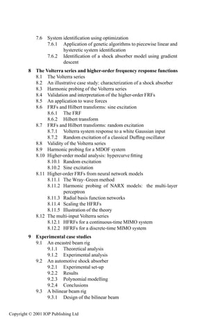
3.12.3 Coulomb friction
In this case
´Ýµ × Ò´Ýµ (3.166)
and equation (3.157) gives
¾
´Øµ ¾ ½ × Ò´ Ó×´ · µµ Ó×´ · µ (3.167)
Ò ¼
so (ignoring , as the integral is over a whole cycle)
¿
¾
¾ ¾
´Øµ ¾ Ó× Ó× (3.168)
Ò ¼ ¾
and
¾ (3.169)
Ò
which integrates trivially to give
¾
´Øµ ¼ Ø (3.170)
Ò
Equation (3.158) gives
½ ¾
´Øµ ¾ × Ò´ Ó× µ × Ò ¼ (3.171)
Ò ¼
so the final solution has
´Øµ ¼ (3.172)
Equation (3.170) shows that the expected form of the decay envelope for a
Coulomb friction system is linear (figure 3.29). This is found to be the case by
simulation or experiment.
It transpires that for SDOF systems at least, the form of the envelope
suffices to fix the form of the nonlinear damping and stiffness functions. The
relevant method of identification requires the use of the Hilbert transform, so the
discussion is postponed until the next chapter.
3.13 Summary
Harmonic balance is a useful technique for deriving the describing functions or
FRFs of nonlinear systems if the nonlinear differential equation of the system is
known. The method of slowly varying amplitude and phase similarly suffices to
estimate the decay envelopes. In fact, many techniques exist which agree with
these methods to the first-order approximations presented in this chapter. Among
them are: perturbation methods [197], multiple scales [196], Galerkin’s method
Copyright © 2001 IOP Publishing Ltd](https://image.slidesharecdn.com/72268096-non-linearity-in-structural-dynamics-detection-identification-and-modelling-copy-120717010202-phpapp02/85/72268096-non-linearity-in-structural-dynamics-detection-identification-and-modelling-copy-141-320.jpg)
![126 FRFs of nonlinear systems
y(t)
t
Figure 3.29. Envelope for SDOF Coulomb friction system.
[76] and normal forms [125]. Useful graphical techniques also exist like the
method of isoclines or Li´ nard’s method [196]. Other more convenient methods
e
of calculating the strength of harmonics can be given, once the Volterra series is
defined in chapter 8.
Copyright © 2001 IOP Publishing Ltd](https://image.slidesharecdn.com/72268096-non-linearity-in-structural-dynamics-detection-identification-and-modelling-copy-120717010202-phpapp02/85/72268096-non-linearity-in-structural-dynamics-detection-identification-and-modelling-copy-142-320.jpg)
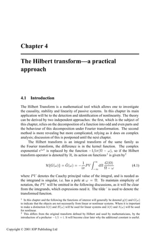
![128 The Hilbert transform—a practical approach
The Hilbert transform and Fourier transform also differ in their
interpretation. The Fourier transform is considered to map functions of time
to functions of frequency and vice versa. In contrast, the Hilbert transform is
understood to map functions of time or frequency into the same domain, i.e.
À ´ µ ´ µ (4.2)
À ´Øµ ´Øµ (4.3)
The Hilbert transform has long been the subject of study by mathematicians,
a nice pedagogical study can be found in [204]. In recent times it has been adopted
as a useful tool in signal processing, communication theory and linear dynamic
testing. A number of relevant references are [24, 43, 49, 65, 81, 89, 105, 116,
126, 130, 151, 210, 211, 247, 255]. The current chapter is intended as a survey
of the Hilbert transform’s recent use in the testing and identification of nonlinear
structures.
4.2 Basis of the method
4.2.1 A relationship between real and imaginary parts of the FRF
The discussion begins with a function of time ´Øµ which has the property that
´Øµ ¼ when Ø ¼. By a slight abuse of terminology, such functions will be
referred to henceforth as causal.
Given any function ´Øµ, there is a decomposition
½ ½
´Øµ Ú Ò´Øµ · Ó ´Øµ ¾ ´ ´Øµ · ´ صµ · ¾ ´ ´Øµ ´ صµ (4.4)
as depicted in figure 4.1. If, in addition, ´Øµ is causal, it follows that
´Øµ ¾ Ø ¼
Ú Ò´Øµ ´Øµ ¾ Ø ¼ (4.5)
and
´Øµ ¾ Ø ¼
Ó ´Øµ ´Øµ ¾ Ø ¼. (4.6)
That this is only true for causal functions is shown by the simple
counterexample in figure 4.2. It follows immediately from equations (4.5) and
(4.6) that
Ú Ò´Øµ Ó ´Øµ ¢ ¯´Øµ (4.7)
Ó ´Øµ Ú Ò´Øµ ¢ ¯´Øµ (4.8)
where ¯´Øµ is the signum function, defined by 3
´
½ Ø ¼
¯´Øµ ¼ Ø ¼ (4.9)
½ Ø ¼.
¿ The notation × Ò´Øµ is often used.
Copyright © 2001 IOP Publishing Ltd](https://image.slidesharecdn.com/72268096-non-linearity-in-structural-dynamics-detection-identification-and-modelling-copy-120717010202-phpapp02/85/72268096-non-linearity-in-structural-dynamics-detection-identification-and-modelling-copy-144-320.jpg)


![Basis of the method 131
So ´ µ, the Fourier transform of a causal ´Øµ, is invariant under the
Hilbert transform and Ê ´ µ and ÁÑ ´ µ are said to form a Hilbert transform
pair. Now, recall from chapter 1 that the impulse response function ´Øµ of a
linear system is causal, this implies that the Fourier transform of ´Øµ—the FRF
À ´ µ—is invariant under Hilbert transformation. It is this property which will be
exploited in later sections in order to detect nonlinearity as FRFs from nonlinear
systems are not guaranteed to have this property.
Further simplifications to these formulae follow from a consideration of the
parity (odd or even) of the functions Ê ´ µ and ÁÑ ´ µ. In fact, Ê ´ µ is
even
½ ½
Ê ´ µ Ø ´Øµ Ó×´ ص Ø ´Øµ Ó×´ ص Ê ´ ص
½ ½
(4.21)
and ÁÑ ´ µ is odd or conjugate-even
½ ½
ÁÑ ´ µ Ø ´Øµ × Ò´ ص Ø ´Øµ × Ò´ ص
½ ½
ÁÑ ´ µ ÁÑ ´ µ (4.22)
where the overline denotes complex conjugation.
Using the parity of ÁÑ ´ µ, equation (4.17) can be rewritten:
½
Ê ´ µ ½ ª
ÁÑ ´ªµ
ª
½
¼ ½ ÁÑ ´ªµ
½ ª
ÁÑ ´ªµ
ª
· ª
ª
½ ¼
½ ÁÑ ´ªµ ½ ÁÑ ´ªµ
½ ª
ª
· ª
ª
¼ ¼
½ ÁÑ ´ ªµ ½ ÁÑ ´ªµ
½ ª
ª · ¼ ª ª
¼
½ ÁÑ ´ªµ ½ ÁÑ ´ªµ
½ ª
ª·
· ª
ª
¼ ¼
½ ÁÑ ´ªµª
¾ ª ¾
ª ¾
(4.23)
¼
and similarly
¾ ½ Ê ´ªµ
ÁÑ ´ µ ª ¾
ª ¾
(4.24)
¼
These equations are often referred to as the Kramers–Kronig relations [154].
The advantage of these forms over (4.17) and (4.18) is simply that the range of
integration is halved and one of the infinite limits is removed.
Copyright © 2001 IOP Publishing Ltd](https://image.slidesharecdn.com/72268096-non-linearity-in-structural-dynamics-detection-identification-and-modelling-copy-120717010202-phpapp02/85/72268096-non-linearity-in-structural-dynamics-detection-identification-and-modelling-copy-147-320.jpg)


![136 The Hilbert transform—a practical approach
4.3.2.1 Conversion to receptance
This correction is only applicable to data with ½ ¼, commonly referred to
as baseband data. The principle is very simple; as the high-frequency decay
of receptance FRF data is faster (Ç´ ¾ µ) than mobility or accelerance data
(Ç´ ½ µ and O(1) respectively), the high-frequency truncation error for the latter
forms of the FRF is reduced by initially converting them to receptance, carrying
out the Hilbert transform, and converting them back. The relations between the
forms are
ÀÁ ´ µ ÀÅ ´ µ ¾ÀÊ ´ µ (4.34)
4.3.2.2 The Fei correction term
This approach was developed by Fei [91] for baseband data and is based on the
asymptotic behaviour of the FRFs of linear systems. The form of the correction
term is entirely dependent on the FRF type; receptance, mobility or accelerance.
As each of the correction terms is similar in principle, only the term for mobility
will be described.
The general form of the mobility function for a linear system with
proportional damping is
Æ
ÀÅ ´ µ ¾ ¾· ¾ (4.35)
½
where is the complex modal amplitude of the th mode; is the undamped
natural frequency of the th mode and is its viscous damping ratio. By
assuming that the damping is small and that the truncation frequency, Ñ Ü , is
much higher than the natural frequency of the highest mode, equation (4.35) can
be reduced to (for Ñ Ü)
Æ
ÀÅ ´ µ (4.36)
½
which is an approximation to the ‘out-of-band’ FRF. This term is purely imaginary
and thus provides a correction for the real part of the Hilbert transform via
equation (4.32). No correction term is applied to the imaginary part as the error
is assumed to be small under the specified conditions.
The actual correction is the integral in equation (4.1) over the interval
´ Ñ Ü ½µ. Hence the correction term, denoted Ê ´ µ, for the real part of the
Hilbert transform is
½ Æ ½
Ê´ µ ¾ ª
ª ÁÑ´ ´ªµµ
ª¾ ¾
¾ ª
ª¾ ¾
(4.37)
ÛÑ Ü ½ Ñ Ü
Copyright © 2001 IOP Publishing Ltd](https://image.slidesharecdn.com/72268096-non-linearity-in-structural-dynamics-detection-identification-and-modelling-copy-120717010202-phpapp02/85/72268096-non-linearity-in-structural-dynamics-detection-identification-and-modelling-copy-152-320.jpg)
![Computation 137
which, after a little algebra [91], leads to
Ê´ µ Ñ Ü ÁÑ´ ´ Ñ Ü µµ
ÐÒ Ñ Ü·
Ñ Ü
(4.38)
4.3.2.3 The Haoui correction term
The second correction term, which again, caters specifically for baseband data,
is based on a different approach. The term was developed by Haoui [130], and
unlike the Fei correction has a simple expression independent of the type of FRF
data used. The correction for the real part of the Hilbert transform is
½
Ê´ µ ¾ ª
ª ÁÑ´ ´ªµµ
ª¾ ¾
(4.39)
ÛÑ Ü
The analysis proceeds by assuming a Taylor expansion for ´ µ about Ñ Ü
and expanding the term ´½ ¾ ª¾ µ ½ using the binomial theorem. If it is
assumed that Ñ Ü is not close to a resonance so that the slope ´ µ (and
higher derivatives) can be neglected, a straightforward calculation yields
Ê´ µ Ê ´¼µ ÁÑ´ ´ Ñ Ü µµ ¾
¾ · ·¡¡¡ (4.40)
ÑÜ ¾ ÑÜ
where Ê ´¼µ is estimated from
ÛÑ
Ê ´¼µ Ê ´ ´¼µµ ¾ Ü
ª
ÁÑ´ ´ªµµ
(4.41)
¼·¯ ª
Using the same approach, the correction term for the imaginary part, denoted
by Á ´ µ, can be obtained:
Á´ Ñ Üµ ¾ ¿
Ê ´ ´ Ñ Ü µµ · ¿ · ·¡¡¡ (4.42)
ÑÜ ¿ ÑÜ ÑÜ
4.3.2.4 The Simon correction method
This method of correction was proposed by Simon [229]; it allows for truncation
at a low frequency, Ñ Ò and a high frequency Ñ Ü . It is therefore suitable for
use with zoomed data. This facility makes the method the most versatile so far.
As before, it is based on the behaviour of the linear FRF, say equation (4.35)
for mobility data. Splitting the Hilbert transform over three frequency ranges:
´¼ Ñ Òµ, ´ Ñ Ò Ñ Ü µ and ´ Ñ Ü ½µ, the truncation errors on the real part of
the Hilbert transform, Ê ´ µ at low frequency and the now familiar Ê ´ µ at
high frequency, can be written as
Ê´ µ ¾ ª ÁÑ´ ´ µµ
ÑÒ
ª
ª¾ ¾
(4.43)
¼
Copyright © 2001 IOP Publishing Ltd](https://image.slidesharecdn.com/72268096-non-linearity-in-structural-dynamics-detection-identification-and-modelling-copy-120717010202-phpapp02/85/72268096-non-linearity-in-structural-dynamics-detection-identification-and-modelling-copy-153-320.jpg)

![Computation 139
ω low ωa ωb ω ri ωc ω d ωhigh
Figure 4.6. Frequency grid for the Ahmed correction term.
Suppose mode is the lowest mode in the measured region with resonant
frequency Ö and therefore has the greatest effect on the low-frequency
truncation error Ê ´ µ, the relevant part of ÁÑ À Ñ can be decomposed:
½
Ñ
ÁÑ ÀÅ ´ µ ¾ ¾ µ¾ · ´ ¾ ¾ µ¾ (4.52)
½´
where the superscript Ñ indicates that this is the mass asymptote of the FRF. In
the lower part of the frequency range is small and the first term can be
expanded:
½ ½ ¾
¾ ¾ µ¾ ½· ·¡¡¡ Ç (4.53)
½´ ½
and neglected, so
Ñ
ÁÑ ÀÅ ´ µ
´ ¾ ¾ µ¾
(4.54)
Now, Ahmed estimates the unknown coefficient by curve-fitting function
(4.54) to the data in the range to where Ñ Ò and
(figure 4.6). (An appropriate least-squares algorithm can be found in [7].) The
low-frequency correction to the Hilbert transform is then found by substituting
(4.51) into the appropriate Kramers–Kronig relation, so
Ê´ µ ¾ ÑÒ
ª¾
ª ¾ µ´ª¾ ¾ µ
´ª¾
(4.55)
¼
Copyright © 2001 IOP Publishing Ltd](https://image.slidesharecdn.com/72268096-non-linearity-in-structural-dynamics-detection-identification-and-modelling-copy-120717010202-phpapp02/85/72268096-non-linearity-in-structural-dynamics-detection-identification-and-modelling-copy-155-320.jpg)


![144 The Hilbert transform—a practical approach
It therefore follows from (4.75) that
½ ´ µ ½ ´ µ ½ ´Øµ¯´Øµ (4.77)
where ¯´Øµ is the signum function defined in (4.9). ( ¯´Øµ ´ µ is proved
in appendix D.)
It immediately follows from (4.77) that
´ µ Æ ¾ Æ ½ ´ µ (4.78)
where the operator ¾ represents multiplication by ¯´Øµ, i.e. ¾ ´Øµ ´Øµ¯´Øµ
and composition is denoted by Æ, i.e. ´ ½ Æ ¾ µ´Øµ ½ ´ ¾ ´Øµµ. In terms of
operators,
À Æ ¾ Æ ½ (4.79)
and the Hilbert transform can therefore be implemented in terms of the Fourier
transform by the three-step procedure:
(1) Take the inverse Fourier transform of ´ µ. This yields the time domain
´Øµ.
(2) Multiply ´Øµ by the signum function ¯´Øµ.
(3) Take the Fourier transform of the product ´Øµ¯´Øµ. This yields the required
Hilbert transform ´ µ.
In practice these operations will be carried out on sampled data, so the
discrete Fourier transform (DFT) or fast Fourier transform will be used. In the
latter case, the number of points should usually be ¾ Æ for some Æ .
The advantage of this method over the direct method described in the
previous section is its speed (if the FFT is used). A comparison was made in
[170]. (The calculations were made on a computer which was extremely slow by
present standards. As a consequence, only ratios of the times have any meaning.)
Number of points 256 512
Direct method 6.0 min 24.1 min
Fourier method 1 1.0 min 2.0 min
The disadvantages of the method arise from the corrections needed. Both
result from the use of the FFT, an operation based on a finite data set.
The first problem arises because the FFT forces periodicity onto the
data outside the measured range, so the function ¯´Øµ which should look like
figure 4.8(a), is represented by the square-wave function ×մص of figure 4.8(b).
This means that the function ´ µ is effectively convolved with the function
ÓØ´ µ ×մص instead of the desired ´ µ. (See [260] for the
appropriate theory.) The effective convolving functions is shown in figure 4.9(b).
Copyright © 2001 IOP Publishing Ltd](https://image.slidesharecdn.com/72268096-non-linearity-in-structural-dynamics-detection-identification-and-modelling-copy-120717010202-phpapp02/85/72268096-non-linearity-in-structural-dynamics-detection-identification-and-modelling-copy-160-320.jpg)
![Computation 145
(a)
ε(t)
+1
t
-1
(b)
sq(t) +1
t
-1
Figure 4.8. Effect of the discrete Fourier transform on the signum function.
As ¼, ÓØ´ µ ´ µ, so for low frequencies or high
sampling rates, the error in the convolution is small. If these conditions are not
met, a correction should be made. The solution is simply to compute the discrete
inverse DFT of the function ´ µ and multiply by that in the time-domain
in place of ¯´Øµ. The problem is that ´ µ is singular at ¼. A naive
approach to the problem is to zero the singular point and take the discrete form 5
of ´ µ:
¼ ½
Æ
Í
´ ½µ ¾
¾ (4.80)
Æ
·½ Æ.
´Æ · ½ µ ¾
The corresponding time function, often called a Hilbert window, is shown
in figure 4.10 (only points Ø ¼ are shown). It is clear that this is a poor
representation of ¯´Øµ. The low-frequency component of the signal between
There are numerous ways of coding the data for an FFT, expression (4.80) follows the conventions
of [209].
Copyright © 2001 IOP Publishing Ltd](https://image.slidesharecdn.com/72268096-non-linearity-in-structural-dynamics-detection-identification-and-modelling-copy-120717010202-phpapp02/85/72268096-non-linearity-in-structural-dynamics-detection-identification-and-modelling-copy-161-320.jpg)
![146 The Hilbert transform—a practical approach
(a)
F [ ε(t) ] = -i
πω
ω
(b)
F [ sq(t) ] = -i cot πω
ω
Figure 4.9. Desired Hilbert window and periodic form from the discrete FFT.
¡ ¾ and ¡ ¾ has been discarded. This can be alleviated by transferring
energy to the neighbouring lines and adopting the definition
¼ ½
¿
¾ ¾
Æ
Í
´ ½µ ¿
¾ (4.81)
Æ
·½ Æ ½
´Æ · ½ µ ¾
¿
Æ.
¾
Copyright © 2001 IOP Publishing Ltd](https://image.slidesharecdn.com/72268096-non-linearity-in-structural-dynamics-detection-identification-and-modelling-copy-120717010202-phpapp02/85/72268096-non-linearity-in-structural-dynamics-detection-identification-and-modelling-copy-162-320.jpg)
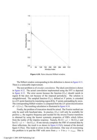

![Computation 149
G (ω)
1
πω
Ideal convolution G(ω) * 1
πω
Figure 4.12. Ideal convolution for the Hilbert transform.
4.3.4 Fourier method 2
Fourier method 1 was discussed as it was the first Hilbert transform method to
exploit Fourier transformation. However, it is rather complicated to implement
and the method discussed in this section is to be preferred in practice.
The implementation of this method is very similar to Fourier method 1;
however, the theoretical basis is rather different. This method is based on the
properties of analytic 6 signals and is attributed to Bendat [24]. Given a time
This terminology is a little unfortunate, as the word analytic will have two different meanings in
this book. The first meaning is given by equation (4.82). The second meaning relates to the pole-zero
structure of complex functions—a function is analytic in a given region of the complex plane if it has
no poles in that region. (Alternatively, the function has a convergent Taylor series.) The appropriate
meaning will always be clear from the context.
Copyright © 2001 IOP Publishing Ltd](https://image.slidesharecdn.com/72268096-non-linearity-in-structural-dynamics-detection-identification-and-modelling-copy-120717010202-phpapp02/85/72268096-non-linearity-in-structural-dynamics-detection-identification-and-modelling-copy-165-320.jpg)


![Computation 153
transform of the real part8 . This fact provides a means of computing the FRF
imaginary part from the real part. In principle, three steps are required:
(1) Take the Fourier transform of the FRF real part Ê ´ µ, i.e. Ê´ µ.
(2) Form the transform ´ µ using (4.89).
(3) Take the inverse Fourier transform ½ of ´ µ. The result is ´ µ, i.e. the
desired Hilbert transform, Ê ´ µ, has been obtained as the imaginary part.
A trivial modification—exchange ÁÑ and Ê —in this argument leads to
the means of computing ÁÑ ´ µ.
One advantage of the method is its speed, the timings are essentially those
of Fourier method 1. Also, because the FFT is applied to a spectrum, which has
already been obtained by FFT and is periodic, there are no leakage effects. The
method is subject to the same truncation problems that afflict all the methods and
the only applicable correction is conversion to receptance. The implementation
of the method is now illustrated by a case study [142].
4.3.5 Case study of the application of Fourier method 2
½
The structure used to obtain the experimental data was a composite ¾¿ scale
aircraft wing used for wind tunnel tests. The wing was secured at its root to a
rigid support, effectively producing a cantilever boundary condition. Excitation
of the wing was via an electrodynamic exciter attached to the wing via a push
rod (stinger) and a force transducer. The excitation was a band-limited random
signal in the range 0–512 Hz. The response of the wing was measured using
lightweight accelerometers. (Note that random excitation is not optimal for
nonlinear structures—this will be discussed later. This study is intended to show
how the Hilbert transform is computed, and one can only validate the method on
a linear structure.)
Figure 4.16 shows the accelerance FRF measured by the experiment. At least
seven modes are visible. For information, the resonance at 76 Hz was identified
as first wing bending, that at 215 Hz was identified as first wing torsion.
Note that
½ ½
Ê ´µ Ø Ó×´ ص ´Øµ Ø Ø
Ú Ò ´Øµ
½ ½
so,
½ ½ Ø
Ê´ µ Ø Ú Ò ´Øµ
½ ½
½ ½ ´ ·Øµ ½
Ø Ú Ò ´Øµ ¾ Ø Ú Ò ´ØµÆ´ · ص
½ ½ ½
¾ Ú Ò ´ µ
So Ê is essentially the even component of the original time signal. This fact does not help with
the development of the algorithm. However, it does show that the terminology ‘pseudo spectrum’ for
Ê, which is sometimes used, is probably inappropriate.
Copyright © 2001 IOP Publishing Ltd](https://image.slidesharecdn.com/72268096-non-linearity-in-structural-dynamics-detection-identification-and-modelling-copy-120717010202-phpapp02/85/72268096-non-linearity-in-structural-dynamics-detection-identification-and-modelling-copy-169-320.jpg)


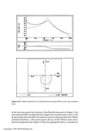

![168 The Hilbert transform—a practical approach
but the characteristic linear Lorentzian shape appears to be retained. In fact,
Volterra series techniques (chapter 8) provide a compelling argument that random
excitation FRFs do change their form for nonlinear systems, but they still do not
show Hilbert transform distortions. Random excitation should not, therefore,
be used if the Hilbert transform is to be used as a diagnostic for detecting
nonlinearity.
The impulse and chirp excitations are intermediate between these two
extremes. They can be used if the test conditions dictate accordingly. Both
methods have the advantage of giving broadband coverage at reasonable speed.
4.6 Indicator functions
The Hilbert transform operations described earlier give a diagnosis of nonlinearity
with a little qualitative information available to those with appropriate experience.
There has in the past been some effort at making the method quantitative. The
FREEVIB approach discussed later actually provides an estimate of the stiffness
or damping functions under certain conditions. There are also a number of
less ambitious attempts which are usually based on computing some statistic or
indicator function which sheds light on the type or extent of nonlinearity. Some
of the more easily computable or interpretable are discussed in the following.
4.6.1 NPR: non-causal power ratio
This statistic was introduced in [141]. It does not make direct use of the Hilbert
transform, but it is appropriate to discuss it here as it exploits the artificial non-
causality of nonlinear system ‘impulse responses’. The method relies on the
decomposition
´Øµ ½ ´ µ Ò ´Øµ · ´Øµ (4.98)
where ´Øµ is the causal part defined by
´Øµ ´Øµ Ø ¼ (4.99)
¼ Ø ¼
and Ҵص is the non-causal part
¼ Ø ¼
Ò ´Øµ ´Øµ Ø ¼. (4.100)
The non-causal power ratio (NPR) is then defined as the ratio of non-causal
power ÈÒ to the total system power È as encoded in the FRF
ʼ
ÈÒ ½ Ø Ò´Øµ ¾
ʽ
NPR
È ½ Ø ´Øµ
¾ (4.101)
Copyright © 2001 IOP Publishing Ltd](https://image.slidesharecdn.com/72268096-non-linearity-in-structural-dynamics-detection-identification-and-modelling-copy-120717010202-phpapp02/85/72268096-non-linearity-in-structural-dynamics-detection-identification-and-modelling-copy-184-320.jpg)
![Indicator functions 169
. .
k3 y3 k3 > 0 c2 y y
.
k3 y3 k3 < 0 F sgn( y)
c
Figure 4.29. Non-causal power ratio plots for various SDOF nonlinear systems.
By Parseval’s theorem, this also has a representation as
ʼ
ÈÒ ½ Ø Ò´Øµ ¾
½Ê½
´ µ¾
NPR (4.102)
È ¾ ½
This index is readily computed using an inverse FFT.
The NPR is, of course, a function of excitation amplitude (the form of the
excitation being dictated by the considerations of the previous section). Kim
and Park [141] compute this function for a number of common nonlinearities:
hardening and softening cubic springs and quadratic and Coulomb damping. It
is argued that the functions are characteristic of the nonlinearity as shown in
figure 4.29, the cubic nonlinearities show NPRs which increase quickly with
amplitude as expected. The NPR for quadratic damping shows a much more
gentle increase, and the Coulomb friction function decreases with amplitude—
again in agreement with intuition. The function certainly gives an indication of
nonlinearity, but claims that it can suggest the type are probably rather optimistic.
The method is not restricted to SDOF systems. A case study is presented in
[141] and it is suggested that computing the NPRs for all elements of the FRF
matrix can yield information about the probable location of the nonlinearity.
Copyright © 2001 IOP Publishing Ltd](https://image.slidesharecdn.com/72268096-non-linearity-in-structural-dynamics-detection-identification-and-modelling-copy-120717010202-phpapp02/85/72268096-non-linearity-in-structural-dynamics-detection-identification-and-modelling-copy-185-320.jpg)
![170 The Hilbert transform—a practical approach
4.6.2 Corehence
This measure of nonlinearity, based on the Hilbert transform, was introduced in
[213] as an adjunct to the coherence function described in chapter 2. The basis of
the theory is the operator of linearity È , defined by 9
´ µ È´ µ ´ µ (4.103)
The operator is the identity È ´ µ ½ if the system is linear (i.e. ´ µ
has a causal inverse Fourier transform). Deviations of È from unity indicate
nonlinearity. Note that È is a function of the level of excitation. As in the case
of the coherence ¾ (chapter 2), it is useful to have a normalized form for the
operator, this is termed the corehence and denoted by ¾ . The definition is10
´ µ ´ µ£ ¾
´ µ¾
´ µ¾ ´ µ¾
(4.104)
There appears to be one major advantage of corehence over coherence.
Given a coherence which departs from unity, it is impossible to determine whether
the departure is the result of nonlinearity or measurement noise. It is claimed in
[213] that this is not the case for corehence, it only responds to nonlinearity. It is
also stated that a coherence of unity does not imply that the system is nonlinear.
However, a rather unlikely type of nonlinearity is needed to create this condition.
It is suggested that the corehence is more sensitive than the coherence.
4.6.3 Spectral moments
Consider a generic time signal ܴص; this has a representation
½ ½ Ø
ܴص ´ µ (4.105)
¾ ½
where ´ µ is the spectrum. It follows that, if ܴص is Ò-times differentiable,
ÒÜ Ò ½
Ò Ø ´ µ (4.106)
ØÒ ¾ ½
½
There are actually a number of È operators, each associated with a different FRF estimator, i.e. À ,
À¾ etc. The results in the text are for the estimator À½ ´ µ ËÝÜ ´ µ ËÜÜ ´ µ.
½¼The actual definition in [213] is
´ µ¾ ´ µ ´ µ£ ¾
´ µ¾ ´ µ¾
However, the expectation operators are implied; if the ´ µ and ´ µ are themselves expectations,
expression (4.104) collapses to unity. There, is therefore, an implicit assumption that the form of
excitation must be random as it is in the case of the coherence. Now, it is stated above that the Hilbert
transform of an FRF obtained from random excitation does not show distortions. This does not affect
the utility of the corehence as that statement only applies to the expectation of the FRF, i.e. the FRF
after averaging. Because £ , the corehence departs from unity for nonlinear
systems.
Copyright © 2001 IOP Publishing Ltd](https://image.slidesharecdn.com/72268096-non-linearity-in-structural-dynamics-detection-identification-and-modelling-copy-120717010202-phpapp02/85/72268096-non-linearity-in-structural-dynamics-detection-identification-and-modelling-copy-186-320.jpg)
![Indicator functions 171
ÒÜ ¬ ½
so
¬ Ò Ò
¬
Ò¬
Ò Å ´Òµ
´ µ (4.107)
Ø Ø ¼ ¾ ½ ¾
where Å ´Òµ denotes the Òth moment integral of ´ µ or the Òth spectral mo-
ʽ
ment— ½ Ò ´ µ. Now it follows from the Taylor’s series
½ ½ ÒÜ ¬
¬ ½ ½ ´Òµ ´ صÒ
ܴص Ò
Ò¬ Ø Å
¬ (4.108)
Ò ½ Ò Ø Ø ¼ ¾ Ò ½ Ò
that the function ܴص is specified completely by the set of spectral moments. As a
result, ´ µ is also specified by this set of numbers. The moments offer a means
of characterizing the shape of the FRF or the corresponding Hilbert transform
in terms of a small set of parameters. Consider the analogy with statistical
theory: there, the mean and standard deviation (first- and second-order moments)
of a probability distribution establish the gross features of the curve. The third-
and fourth-order moments describe more subtle features—the skewness and the
‘peakiness’ (kurtosis). The latter features are considered to be measures of the
distortion from the ideal Gaussian form. The zeroth moment is also informative;
this is the energy or area under the curve.
Assuming that the moments are estimated for a single resonance between
Ñ Ò and Ñ Ü , the spectral moments of an FRF ´ µ are
Å ´Òµ
Ñ Ü
Ò ´ µ (4.109)
ÑÒ
Note that they are complex, and in general depend on the limits; for consistency,
the half-power points are usually taken. The moments are approximated in
practice by
Å ´Òµ
Ñ Ü
Ò ´ µ¡ (4.110)
ÑÒ
where ¡ is the spectral line spacing.
So-called Hilbert transform describers—HTDs—are then computed from
Å ´Òµ Å ´Òµ
HTD´Òµ ½¼¼
Å ´Òµ
(4.111)
and these are simply the percentage differences between the Hilbert transform
moments and the original FRF moments.
In practice, only the lowest-order moments have been investigated; in the
terminology of [145], they are
real energy ratio (RER) Ê HTD ´¼µ
imaginary energy ratio (IER) ÁÑ HTD ´¼µ
real frequency ratio (RFR) Ê HTD ´½µ
Copyright © 2001 IOP Publishing Ltd](https://image.slidesharecdn.com/72268096-non-linearity-in-structural-dynamics-detection-identification-and-modelling-copy-120717010202-phpapp02/85/72268096-non-linearity-in-structural-dynamics-detection-identification-and-modelling-copy-187-320.jpg)

![Measurement of apparent damping 173
Figure 4.30 shows the plots of the HTD statistics as a function of applied
force for several common nonlinearities. The parameters appear to separate
stiffness and damping nonlinearities very effectively. Stiffness nonlinearity is
identified from the changes in the RFR and IAR, while damping nonlinearity
is indicated by changes in the energy statistics without change in the other
describers. Note that the describers tend to zero at low forcing for the polynomial
nonlinearities as expected; in this region. For the discontinuous
nonlinearities, clearance and friction, the describers tend to zero at high forcing
as the behaviour near the discontinuities becomes less significant. The describers
therefore indicate the level of forcing at which the FRF of the underlying linear
system can be extracted.
4.7 Measurement of apparent damping
It is well known that the accurate estimation of damping for lightly damped and/or
nonlinear structures presents a difficult problem. In the first case, traditional
methods of curve-fitting to FRFs break downÔ to low resolution of the peaks.
due
In the second case, the damping ratio ¾ Ñ is not constant, whether the
nonlinearity is in stiffness or damping (as a result, the term apparent damping
ratio is used). However, it transpires that there is an effective procedure based
on the Hilbert transform [245], which has actually been implemented on several
commercial FRF analyers. The application to light damping is discussed in [4, 5].
Investigations of nonlinear systems are presented in [187, 188].
The basis of the method is the analytic signal. Consider the function
´ · µØ with ¼. It is shown in appendix C that there are relations between
the real and imaginary parts:
À Ø × Ò´ ص Ø Ó×´ ص (4.113)
and
À Ø Ó×´ ص Ø × Ò´ ص (4.114)
provided is small. These relations therefore apply to the impulse response of a
linear system provided the damping ratio is small (overall constant factors have
no effect):
½ ÒØ
´Øµ × Ò´ ص Ø ¼ (4.115)
Ñ
which can be interpreted as the real part of an analytic signal,
½ ½
´Øµ ´Øµ ´Øµ ÒØ × Ò´ ص ÒØ Ó×´ ص
Ñ Ñ
´ Ò · µØ (4.116)
Ñ
Copyright © 2001 IOP Publishing Ltd](https://image.slidesharecdn.com/72268096-non-linearity-in-structural-dynamics-detection-identification-and-modelling-copy-120717010202-phpapp02/85/72268096-non-linearity-in-structural-dynamics-detection-identification-and-modelling-copy-189-320.jpg)

![Identification of nonlinear systems 175
Figure 4.31. Impulse response and envelope function for a nonlinear system under random
excitation: (a) low level; (b) high level.
An experimental example for an impacting cantilever beam (figure 4.33) also
shows the utility of the method. Figure 4.34 shows the FRF, impulse response
and log envelope for the low excitation case where the system does not impact.
Figure 4.35 shows the corresponding plots for the high-excitation contacting
case—note that the FRF is considerably noisier. If the initial, linear, portions of
the log envelope curves are used for regression, the resulting natural frequencies
and damping ratios are given in figure 4.36.
Ô
The apparent variation in damping ratio is due to the fact that the definition
Ñ depends on the nonlinear stiffness. The corresponding value of
should be constant (by linearization arguments presented in chapter 2).
4.8 Identification of nonlinear systems
The method described in this section is the result of a programme of research by
Feldman [92, 93, 94]. It provides a means of obtaining the stiffness and damping
Copyright © 2001 IOP Publishing Ltd](https://image.slidesharecdn.com/72268096-non-linearity-in-structural-dynamics-detection-identification-and-modelling-copy-120717010202-phpapp02/85/72268096-non-linearity-in-structural-dynamics-detection-identification-and-modelling-copy-191-320.jpg)


![182 The Hilbert transform—a practical approach
is taken of (4.120), it will pass through the functions and ¾
¼. Further, the
transform commutes with differentiation (appendix C again), so
¾
Ý · ´ØµÝ · ¼ ´ØµÝ ¼ (4.130)
Adding (4.120) and (4.130) yields a differential equation for the analytic
signal , i.e.
· ´Øµ · ¼ ´Øµ¾ ¼ (4.131)
or, the quasi-linear form,
¾
· ´ µ · ¼´ µ ¼ (4.132)
Now, the derivatives and are known functions of and by (4.128)
and (4.129). Substitution yields
¾· ¼·
¾ · ¾ · · ¼ (4.133)
Separating out the real and imaginary parts gives
´Øµ ¾ (4.134)
¾
¼ ´Øµ ¾ (4.135)
or
¾ ¾ ¾
¼ ´Øµ ·¾ ¾ · (4.136)
and these are the basic equations of the theory.
On to practical matters. Suppose the free vibration is induced by an impulse,
the subsequent response of the system will take the form of a decay. Ý ´Øµ can
be measured and Ý can then be computed 12. This means that ´Øµ and ´Øµ are
available by using (4.124) and (4.125) and numerically differentiating ´Øµ.
Now, consider how the damping function is obtained. ´Øµ is known from
(4.134). As ´Øµ is monotonically decreasing (energy is being dissipated), the
inverse function Ø´ µ is single-valued and can be obtained from the graph of
´Øµ against time (figure 4.37). The value of ´ µ is simply the value of ´Øµ
at Ø´ µ (figure 4.38). Similarly, the stiffness function is obtained via the sequence
¾ ¾
Ø´ µ ¼ ´Ø´ µµ ¼ ´ µ. The inverse of the latter mapping ´ µ
is sometimes referred to as the backbone curve of the system. (For fairly simple
systems like the Duffing oscillator, the backbone curves can be calculated [41].)
½¾ As in the frequency-domain case, there are a number of methods of computing Ý, the decomposition
À ½ Æ ¾ Æ provides one.
Copyright © 2001 IOP Publishing Ltd](https://image.slidesharecdn.com/72268096-non-linearity-in-structural-dynamics-detection-identification-and-modelling-copy-120717010202-phpapp02/85/72268096-non-linearity-in-structural-dynamics-detection-identification-and-modelling-copy-198-320.jpg)


![Identification of nonlinear systems 187
e f
8000 600
6000
400
4000
200
2000
Damping force
Spring force
0 0
−2000
−200
−4000
−400
−6000
−8000 −600
−1 −0.5 0 0.5 1 −100 −50 0 50 100
Displacement Velocity
Figure 4.40. (Continued)
simple methods suffice to estimate the stiffness function.) Note that because the
initial displacement did not decay away completely, there are gaps in the stiffness
and damping functions at low amplitude.
The final example shows a damping nonlinearity. The system has equation
of motion
Ý · ¿¼¼ × Ò´Ýµ · ½¼ Ý ¼ (4.142)
so Coulomb friction is present. The decay began with the same initial conditions
as before and the resulting anlysis is shown in figures 4.41(a)–(f ). Note the
characteristic linear decay envelope for this type of nonlinear system as shown
in figure 4.41(a). In this case, the backbone (figure 4.41(c)) shows no variation of
natural frequency with amplitude as expected. The coefficient of friction can be
read directly from the damping function (figure 4.41(f )).
Further examples of nonlinear systems can be found in [93, 95]. A practical
application to a nonlinear ocean mooring system is discussed in [120].
All of these examples have viscous damping models. It is a simple matter to
modify the theory for structural (hysteretic) damping, the equation of motion for
the analytic signal becomes
¾
· ¼ ´ µ ½ · Æ´ µ ¼ (4.143)
where Æ ´ µ is the loss factor or logarithmic decrement. The basic equations are
¾
¼ ´Øµ ¾ (4.144)
Copyright © 2001 IOP Publishing Ltd](https://image.slidesharecdn.com/72268096-non-linearity-in-structural-dynamics-detection-identification-and-modelling-copy-120717010202-phpapp02/85/72268096-non-linearity-in-structural-dynamics-detection-identification-and-modelling-copy-203-320.jpg)

![Identification of nonlinear systems 189
4
x 10 e f
3
600
2 400
1 200
Damping force
Spring force
0 0
−1 −200
−2 −400
−600
−3
−4 −2 0 2 4 −200 −100 0 100 200
Displacement Velocity
Figure 4.41. (Continued)
and
ƴص ¾ ¾ ¾ (4.145)
¼ ¼
The method described here is only truly suitable for monocomponent signals,
i.e. those with a single dominant frequency. The extension to two-component
signals is discussed in [96].
4.8.2 FORCEVIB
The analysis for the forced vibration case is very similar to FREEVIB; the
presence of the excitation complicates matters very little. Under all the same
assumptions as before, the quasi-linear equation of motion for the analytic signal
can be obtained:
¾
· ´ µ · ¼´ µ (4.146)
Ñ
Carrying out the same procedures as before which lead to equations (4.134) and
(4.135) yields
¬ ´Øµ
´Øµ
Ñ
¾ (4.147)
and
¾ ¾ · «´Øµ ¬ ´Øµ ¾
¼ ´Øµ Ñ Ñ
·¾ ¾ · (4.148)
Copyright © 2001 IOP Publishing Ltd](https://image.slidesharecdn.com/72268096-non-linearity-in-structural-dynamics-detection-identification-and-modelling-copy-120717010202-phpapp02/85/72268096-non-linearity-in-structural-dynamics-detection-identification-and-modelling-copy-205-320.jpg)
![190 The Hilbert transform—a practical approach
where «´Øµ and ¬ ´Øµ are, respectively, the real and imaginary parts of the
input/output ratio , i.e.
´Øµ ܴصݴص · ܴصݴص ܴصݴص ܴصݴص
«´Øµ · ¬ ´Øµ ·
ݾ ´Øµ · ݾ ´Øµ ݾ ´Øµ · ݾ ´Øµ
(4.149)
´Øµ
where ܴص is the real part of ´Øµ, i.e. the original physical excitation.
Implementation of this method is complicated by the fact that an estimate of
the mass Ñ is needed. This problem is discussed in detail in [94].
4.9 Principal component analysis (PCA)
This is a classical method of multivariate statistics and its theory and use are
documented in any textbook from that field (e.g. [224]). Only the briefest
description will be given here. Given a set of Ô-dimensional vectors Ü
´Ü½ ÜÔ µ, the principal components algorithm seeks to project, by a linear
transformation, the data into a new Ô-dimensional set of Cartesian coordinates
´Þ½ Þ¾ ÞÔµ. The new coordinates have the following property: Þ ½ is the linear
combination of the original Ü with maximal variance, Þ ¾ is the linear combination
which explains most of the remaining variance and so on. It should be clear
that, if the Ô-coordinates are actually a linear combination of Õ Ô variables,
the first Õ principal components will completely characterize the data and the
remaining Ô Õ will be zero. In practice, due to measurement uncertainty, the
principal components will all be non-zero and the user should select the number
of significant components for retention.
Calculation is as follows: given data Ü ´Ü½ ܾ Ü Ôµ
½ Æ , form the covariance matrix ¦ (see appendix A—here the factor
½ ´Æ ½µ is irrelevant)
Æ
¦ ´ Ü Ü µ´ Ü Ü µÌ (4.150)
½
(where Ü is the vector of means of the Ü data) and decompose so
£ Ì (4.151)
where £ is diagonal. (Singular value decomposition can be used for this step
[209].) The transformation to principal components is then
Þ Ì´ Ü Ü µ (4.152)
Considered as a means of dimension reduction then, PCA works by
discarding those linear combinations of the data which contribute least to
the overall variance or range of the data set. Another way of looking at
the transformation is to consider it as a means of identifying correlations or
Copyright © 2001 IOP Publishing Ltd](https://image.slidesharecdn.com/72268096-non-linearity-in-structural-dynamics-detection-identification-and-modelling-copy-120717010202-phpapp02/85/72268096-non-linearity-in-structural-dynamics-detection-identification-and-modelling-copy-206-320.jpg)
![Principal component analysis (PCA) 191
Magnitude
Frequency (Hz)
Phase (rad)
Frequency (Hz)
Figure 4.42. FRF À½ for symmetric 2DOF linear system.
redundancy in data. The transformation to principal components results in
uncorrelated vectors and thus eliminates the redundancy.
The first applications of the method in dynamics date back to the early 1980s.
One of the first references is by Moore [191]. The first applications in modal
testing or structural dynamics are due to Leuridan [163, 164]. In both cases, the
object of the exercise was model reduction.
Consider a structure instrumented with Ô sensors, say measuring
displacement. At each time instant Ø, the instrumentation returns a vector
of measurements Ý ´Øµ ´Ý´Øµ½ Ý´ØµÔ µ. Because of the dynamical
interactions between the coordinates there will be some correlation and hence
redundancy; using PCA this redundancy can potentially be eliminated leaving
a lower dimensional vector of ‘pseudo-sensor’ measurements which are linear
Copyright © 2001 IOP Publishing Ltd](https://image.slidesharecdn.com/72268096-non-linearity-in-structural-dynamics-detection-identification-and-modelling-copy-120717010202-phpapp02/85/72268096-non-linearity-in-structural-dynamics-detection-identification-and-modelling-copy-207-320.jpg)


![Principal component analysis (PCA) 199
0.0003
X = 1.0
X = 5.0
X = 10.0
0.0002
Receptance
0.0001
0.0000
0.0 10.0 20.0 30.0 40.0 50.0 60.0
Frequency (Hz)
Figure 4.52. Principal FRF È £¾ for symmetric 2DOF nonlinear system at low medium
and high excitation.
with infinite ranges. In practice, the covariance matrices are computed using
finite summations. In the time-domain case, this presents no serious problems
in applying (4.153) as long as the records are long enough that the means of the
signals approximate to zero. However, in the frequency domain, the FRFs are
not zero-mean due to the finite frequency range. This means that the covariance
matrix in (4.162) is inappropriate to decorrelate the FRF vector. The remedy is
simply to return to equation (4.150) and use the covariance matrix
Æ ¾
¦ ´ À´ µ À ´ µ µ´ À ´ µ À ´ µ µÌ (4.163)
½
Using this prescription gives the principal FRFs shown in figures 4.46 and
4.47. This time the principal component transformation has produced modal
FRFs. Unfortunately, this situation is not generic. It is the result here of
considering a system with a high degree of symmetry; also the mass matrix is
unity and this appears to be critical. Figure 4.48 shows the principal FRFs for
a system identical to (4.160) and (4.161) except that the two equations have
different mass values—the decoupling property has been lost even though the
modal transformation can still achieve this. However, throughout the development
of the PCA method it was hoped that the principal FRFs would generally exhibit
some simplification.
In terms of nonlinear systems, the aim of PCA (or as it is sometimes called—
the Karhunen–Loeve expansion [257]) is to hopefully localize the nonlinearity in
a subset of the responses. By way of illustration consider the system in (4.160)
and (4.161) supplemented by a cubic stiffness nonlinearity connecting the two
Copyright © 2001 IOP Publishing Ltd](https://image.slidesharecdn.com/72268096-non-linearity-in-structural-dynamics-detection-identification-and-modelling-copy-120717010202-phpapp02/85/72268096-non-linearity-in-structural-dynamics-detection-identification-and-modelling-copy-215-320.jpg)

![Principal component analysis (PCA) 201
Magnitude
Frequency (Hz)
Phase (rad)
Frequency (Hz)
Figure 4.54. Principal FRF È £¾ for symmetric 2DOF nonlinear system with Hilbert
transform.
The reason for the presence of this section in this chapter is that any test
for nonlinearity can be applied to the principal FRFs including of course the
Hilbert transform. This has been studied in the past by Ahmed [7] amongst
others. Figures 4.53 and 4.54 show the result of applying the Hilbert transform
to the principal FRFs for the system discussed earlier. As one might expect, the
nonlinearity is only flagged for the second mode.
With that brief return to the Hilbert transform the chapter is concluded.
The Hilbert transform has been seen to be a robust and sensitive indicator of
nonlinearity. It is a little surprising that it has not yet been adopted by suppliers
of commercial FRF analysers. The next chapter continues the Hilbert transform
theme by considering an approach to the analysis which uses complex function
theory.
Copyright © 2001 IOP Publishing Ltd](https://image.slidesharecdn.com/72268096-non-linearity-in-structural-dynamics-detection-identification-and-modelling-copy-120717010202-phpapp02/85/72268096-non-linearity-in-structural-dynamics-detection-identification-and-modelling-copy-217-320.jpg)
![Chapter 5
The Hilbert transform—a complex
analytical approach
5.1 Introduction
The previous chapter derived the Hilbert transform and showed how it could be
used in a number of problems in engineering dynamics and in particular how it
could be used to detect and identify nonlinearity. It was clear from the analysis
that there is a relationship between causality of the impulse response function and
the occurrence of Hilbert transform pairs in the FRF. In fact, this relationship is
quite deep and can only be fully explored using the theory of complex functions.
Because of this, the mathematical background needed for this chapter is more
extensive than for any other in the book with the exception of chapter 8. However,
the effort is worthwhile as many useful new results become available. There
are many textbooks on complex analysis which provide the prerequisites for this
chapter: [6] is a classic text which provides a rigorous approach, while [234]
provides a more relaxed introduction. Many texts on engineering mathematics
cover the relevant material; [153] is a standard.
5.2 Hilbert transforms from complex analysis
The starting point for this approach is Cauchy’s theorem [234], which states:
given a function (where denotes the complex plane) and
a simple closed contour such that is analytic 1 on and inside , then
½ ´ªµ
ª ¼
ª
(5.1)
¾
if and only if lies outside .
½ Not analytic in the signal sense, meaning that the function has no poles, i.e. singularities.
Copyright © 2001 IOP Publishing Ltd](https://image.slidesharecdn.com/72268096-non-linearity-in-structural-dynamics-detection-identification-and-modelling-copy-120717010202-phpapp02/85/72268096-non-linearity-in-structural-dynamics-detection-identification-and-modelling-copy-218-320.jpg)
![Hilbert transforms from complex analysis 203
v
-R R
u
ω = u - iv
R
R
Figure 5.1. Main contour for deriving the Hilbert transform relation.
The derivation requires that the value of the integral be established (1) when is
inside and (2) when is on :
(1) inside . In this case one can use Cauchy’s calculus of residues [234] to
find the value of the integral, i.e.
½ ´ªµ ´ªµ
ª Ê×
ª ª
(5.2)
¾ ÈÓÐ ×
and, in this case, there is a single simple pole at ª , so the residue is
given by
´ªµ
ª Ñ ´ª µ ¢ ª
Ð (5.3)
So
½ ´ªµ
ª ´ µ
ª
(5.4)
¾
(2) on . In all the cases of interest for studying the Hilbert transform, only
one type of contour is needed; so, for the sake of simplicity, the results that
follow are established using that contour. The argument follows closely that
of [193]. Consider the contour in figure 5.1. Initially Ù Ú is below
the real axis and the residue theorem gives
½ Ê ´ªµ
´ µ ´Ù Ú µ ª ·Á
¾ Ê ª Ù · Ú
(5.5)
Copyright © 2001 IOP Publishing Ltd](https://image.slidesharecdn.com/72268096-non-linearity-in-structural-dynamics-detection-identification-and-modelling-copy-120717010202-phpapp02/85/72268096-non-linearity-in-structural-dynamics-detection-identification-and-modelling-copy-219-320.jpg)
![204 The Hilbert transform—a complex analytical approach
c = Semicircle of radius r
Ω=u
- 1
0 +
Figure 5.2. Contour deformation used to avoid the pole on the real axis.
where Á is the semi-circular part of the contour. If now Ê ½ under
the additional assumption that ´ªµ ´ª µ tends to zero as ª ½ fast
enough to make Á vanish2 , the result is
½ ½ ´ªµ
´ µ ´Ù Úµ ª
¾ ½ ª Ù · Ú
(5.6)
In order to restrict the integrand in (5.5) to real values, one must have Ú ¼
or Ù. However, in order to use the results previously established,
should lie off the contour—in this case the real axis. The solution to this
problem is to deform the contour by adding the section ¼ as shown in
figure 5.2. ¼ is essentially removed by allowing its radius Ö to tend to zero
after has moved onto the real axis. Equation (5.5) becomes (on taking the
integration anticlockwise around the contour)
¾ ´ µ ¾ Ú Ñ ´Ù Úµ
Ð ¼ (5.7)
·Ö ´ªµ ½ ´ªµ
ÖÐ Ñ Ú Ñ
¼ Ð ¼ ½
ª
ª Ù· Ú
· ª
Ö ª Ù · Ú
´ªµ
· ª
ª Ù· Ú
(5.8)
¼
Taking the first limit and changing to polar coordinates on the small semi-
circle yields
·Ö ´ªµ ½ ´ªµ
¾ ´ µ ÖÐ Ñ ª · ª
¼ ½ ª Ö ª
´ ·Ö µ
· ´ ·Ö µ (5.9)
¼ Ö
½ ´ªµ
ÈÎ ª · ´ µ
½ ª
(5.10)
¾ For example, suppose that ´ªµ is Ç´Ê ½ µ as Ê ½, then the integrand is Ç´Ê ¾ µ and the
integral Á is Ê ¢ Ç´Ê ¾ µ Ç´Ê ½ µ and therefore tends to zero as Ê ½. This is by no
means a rigorous argument, consult [234] or any introductory book on complex analysis.
Copyright © 2001 IOP Publishing Ltd](https://image.slidesharecdn.com/72268096-non-linearity-in-structural-dynamics-detection-identification-and-modelling-copy-120717010202-phpapp02/85/72268096-non-linearity-in-structural-dynamics-detection-identification-and-modelling-copy-220-320.jpg)
![Titchmarsh’s theorem 205
where È Î denotes the Cauchy principal value defined by
½ Ö ½
ÈÎ ª ´ªµ ÖРѼ ª ´ªµ · ª ´ªµ (5.11)
½ ½ ·Ö
in the case that ´ªµ has a pole at ª .
The final result of this analysis is
½ ´ªµ
´ µ È Î ª
ª
ª¾Ê (5.12)
½
In pure mathematics, as discussed in the previous chapter, the Hilbert
Transform À of a function is defined by
½ ½ ´ªµ
À ´ µ ÈÎ ª
ª
(5.13)
½
so equation (5.12) can be written in the more compact form
´ µ À ´ µ (5.14)
Equation (5.14) is the desired result. It is important to bear in mind the
assumptions made in its derivation, namely
(1) is analytic in the area bounded by the contour . In the limit above as
Ê ½, this is the lower complex half-plane.
(2) ´ µ tends to zero fast enough as Ê ½ for the integral Á to vanish.
It is convenient (and also follows the conventions introduced somewhat
arbitrarily in the last chapter) to absorb the factor into the definition of the
Hilbert transform. In which case equation (5.14) becomes
´ µ À ´ µ (5.15)
as in equation (4.20). This is a fascinating result—the same condition is obtained
on the class of functions analytic in the lower half-plane as was derived for
transfer functions whose impulse responses are causal. This is not a coincidence;
the reasons for this correspondence will be given in the next section.
5.3 Titchmarsh’s theorem
The arguments of the previous section are expressed rigorously by Titchmarsh’s
theorem which is stated here in its most abstract form (taken from [118]).
Theorem. If ´ µ is the Fourier transform of a function which vanishes for Ø ¼
and ½
´ µ¾ ½ (5.16)
½
Copyright © 2001 IOP Publishing Ltd](https://image.slidesharecdn.com/72268096-non-linearity-in-structural-dynamics-detection-identification-and-modelling-copy-120717010202-phpapp02/85/72268096-non-linearity-in-structural-dynamics-detection-identification-and-modelling-copy-221-320.jpg)


![208 The Hilbert transform—a complex analytical approach
Carrying out a long division on (5.27) yields
Ò ¼´ µ
´ µ · (5.29)
Ò ´ µ
where ¼ is a polynomial of order Ò ½. In other words,
¼´ µ
´ µ ½ ´ µ Ò (5.30)
Ò ´ µ
and ¼ ´ µ ´ µ is Ç´ ½ µ as ½. This means that ¼ ´ µ ´ µ is square-
integrable and therefore satisfies the conditions of Titchmarsh’s theorem. Hence,
¼´ µ ½ ¼ ´ªµ ½
´ µ
½ ª
´ªµ ª
(5.31)
½
or ½ ´ªµ ½
´ µ ½ ½ ª
ª
(5.32)
½
So if a function fails to satisfy the conditions required by Titchmarsh’s
theorem because of asymptotically constant behaviour, subtracting the limiting
value produces a valid function. The relations between real and imaginary parts
(4.17) and (4.18) are modified as follows:
½ ÁÑ ´ªµ ÁÑ ½
Ê ´ µ Ê ½ ½ ª
ª
(5.33)
½
½ ½ Ê ´ªµ Ê ½
ÁÑ ´ µ ÁÑ ½ · ª
ª
(5.34)
½
These equations are well known in physical optics and elementary particle
physics. The first of the pair produces the Kramers–Kronig dispersion relation
if ´ µ is taken as Ò´ µ—the complex refractive index of a material. The term
‘dispersion’ refers to the variation of the said refractive index with frequency of
incident radiation [77].
One possible obstruction to the direct application of equations (5.32)–(5.34)
is that ´ µ is usually an experimentally measured quantity. It is clear that ½
will not usually be available. However, this problem can be solved by using a
subtraction scheme as follows. Suppose for the sake of simplicity that the limiting
value of ´ µ as ½ is real and that a measurement of is available at
« ½. Equation (5.33) yields
½
Ê ´ µ Ê ½ ½ ª
ÁÑ ´ªµ
ª
(5.35)
½
and at « this becomes
½
Ê ´«µ Ê ½ ½ ª
ÁÑ ´ªµ
ª «
(5.36)
½
Copyright © 2001 IOP Publishing Ltd](https://image.slidesharecdn.com/72268096-non-linearity-in-structural-dynamics-detection-identification-and-modelling-copy-120717010202-phpapp02/85/72268096-non-linearity-in-structural-dynamics-detection-identification-and-modelling-copy-224-320.jpg)
![Correcting for bad asymptotic behaviour 209
and subtracting (5.36) from (5.35) yields
½
Ê ´ µ Ê ´«µ ½ ª
½
ª
½
ª « ÁÑ ´ªµ (5.37)
½
or
½
Ê ´ µ Ê ´«µ ´ «µ ª
ÁÑ ´ªµ
´ª µ´ª «µ
(5.38)
½
Note that in compensating for lack of knowledge of ½ , the analysis has
produced a more complicated integral. In general if ´ µ behaves as some
polynomial as ½, a subtraction strategy will correct for the bad asymptotic
behaviour in much the same way as before. Unfortunately, each subtraction
complicates the integral further.
The application of these formulae will now be demonstrated in a number of
case studies.
5.4.1 Simple examples
The first pair of case studies allow all the relevant calculations to be carried out
by hand.
The first example calculation comes from [215]. The object of the paper was
to demonstrate a nonlinear system which was nonetheless causal and therefore
satisfied Hilbert transform relations. The system under study was a simple
squaring device 4 , i.e. Ý ´Øµ ܴص¾ . The excitation was designed to give no
response at negative times, i.e.
Ø Ø ¼, ¼
ܴص (5.39)
¼ Ø ¼.
A type of FRF was defined by dividing the spectrum of the output by the
spectrum of the input:
´ µ ¾ ¾ Ø ´ µ
£´ µ
´ µ Ø ´ ¾ µ
(5.40)
so
´ ¾ · ¾ ¾µ
Ê £´ µ ¾· ¾ ÁÑ £´ µ ¾· ¾ (5.41)
As a remark for the sophisticate or person who has read later chapters first, it does not really make
sense to consider this system for this purpose as it does not possess a linear FRF. If the system is
excited with a pure harmonic Ø the response consists of a purely second order part ¾ Ø ; thus
´
À¾ ½ ¾ µ ½ and ÀÒ ¼ ¾
Ò . As the system has no À½ , it has no impulse response ½ and
therefore discussions of causality do not apply.
Copyright © 2001 IOP Publishing Ltd](https://image.slidesharecdn.com/72268096-non-linearity-in-structural-dynamics-detection-identification-and-modelling-copy-120717010202-phpapp02/85/72268096-non-linearity-in-structural-dynamics-detection-identification-and-modelling-copy-225-320.jpg)

![Correcting for bad asymptotic behaviour 211
k c
y(t)
x(t)
Figure 5.3. A first-order dynamical system.
the Æ -function is the time-domain analogue of correcting for the bad asymptotic
behaviour in the frequency domain.
Another example of this type of calculation occurs in [122]. The first-order
linear system depicted in figure 5.3 is used to illustrate the theory. The system has
¾
the FRF
À´ µ
· ¾ ¾· ¾ ¾ ¾· ¾ (5.50)
It is correctly stated that
½ ½ Ê À´ µ
ÁÑ À ´ µ ª ¾ ¾· ¾
ª
(5.51)
½
i.e. the relation in (4.18) applies. However, because
½
РѽÀ ´ µ
¼ (5.52)
the appropriate formula for calculating Ê À ´ µ from ÁÑ À ´ µ is (5.33), i.e.
½ ½ ÁÑ À ´ µ
Ê À´ µ · ½ ª
ª
(5.53)
½
5.4.2 An example of engineering interest
Consider the linear system
ÑÝ · Ý · Ý Ü´Øµ (5.54)
Ê
The integrals involve terms of the form ª ´ª µ which are proportional to ÐÓ ´ ½µ. If the
principal sheet of the ÐÓ function is specified, these terms can be disregarded.
Copyright © 2001 IOP Publishing Ltd](https://image.slidesharecdn.com/72268096-non-linearity-in-structural-dynamics-detection-identification-and-modelling-copy-120717010202-phpapp02/85/72268096-non-linearity-in-structural-dynamics-detection-identification-and-modelling-copy-227-320.jpg)


![Hysteretic damping models 217
half-plane and therefore satisfies the conditions of Titchmarsh’s theorem in .
This means that the zeros of the denominator (assume a SDOF system)
´ µ Ñ ¾ · · (5.74)
are in the upper half-plane. If the conventions are changed to · , the denominator
changes to
·´ µ Ñ ¾ · (5.75)
i.e. the product of the roots remains the same while their sum changes sign.
Clearly the roots of · ´ µ are in the lower half-plane as required by the ·
Titchmarsh theorem.
5.6 Hysteretic damping models
Having established the connection between causality and FRF pole structure, now
is a convenient time to make some observations about the different damping
models used with FRFs. The two main models in use are the viscous damping
model as discussed in chapter 1, where the receptance FRF takes the form
½
À´ µ
Ñ´ Ò ¾ · ¾
¾ (5.76)
Ò µ
and the hysteretic or structural damping model whose FRF has the form [87]
½
À´ µ
Ñ´ Ò ´½ · µ ¾ µ
¾ (5.77)
where is the hysteretic or structural damping loss factor. (The discussion can
be restricted to SDOF systems without losing generality.)
It is shown in chapter 1 that the viscous damping model results in a causal
impulse response and therefore constitutes a physically plausible approximation
to reality. The corresponding calculations for the hysteretic damping model
follow.
Before explicitly calculating the impulse response, the question of its
causality can be settled by considering the pole structure of (5.77). The poles
are at ¦ , where
Ò ´½ · µ ¾
½
(5.78)
A short calculation shows that
ÁÑ ½ · ½ ´½ · ¾ µ µ
Ò ´ ¾
½ ½
¾ ¾ ¾ (5.79)
so if ¼, it follows that
½ ´½ · ¾ µ ½½
¼
¾ ¾¾ (5.80)
Copyright © 2001 IOP Publishing Ltd](https://image.slidesharecdn.com/72268096-non-linearity-in-structural-dynamics-detection-identification-and-modelling-copy-120717010202-phpapp02/85/72268096-non-linearity-in-structural-dynamics-detection-identification-and-modelling-copy-233-320.jpg)
![218 The Hilbert transform—a complex analytical approach
Im ω
ω2
Im λ > 0
Re λ Re ω
ω1
Figure 5.8. Poles of an FRF with hysteretic damping.
and has a non-zero imaginary part. This gives the pole structure shown in
figure 5.8. À ´ µ in equation (5.77) therefore fails to be analytic in either half-
plane. It can be concluded that the impulse response corresponding to this À ´ µ is
non-causal. The next question concerns the extent to which causality is violated;
if the impulse response is small for all Ø ¼, the hysteretic damping model may
still prove useful.
The next derivation follows that of [7], which in turn follows [185]. Recall
that the impulse response is defined by
½ ½ ØÀ ´
´Øµ µ (5.81)
¾ ½
It is a simple matter to show that reality of ´Øµ implies a conjugate symmetry
constraint on the FRF
À ´ µ À £´ µ (5.82)
On making use of this symmetry, it is possible to cast the impulse response
expression in a slightly different form
½ ½
´Øµ Ê ØÀ ´ µ (5.83)
¼
which will prove useful. Note that the expression (5.77) does not satisfy the
conjugate symmetry constraint. To obtain an expression valid on the interval
Copyright © 2001 IOP Publishing Ltd](https://image.slidesharecdn.com/72268096-non-linearity-in-structural-dynamics-detection-identification-and-modelling-copy-120717010202-phpapp02/85/72268096-non-linearity-in-structural-dynamics-detection-identification-and-modelling-copy-234-320.jpg)
![Hysteretic damping models 219
½ ½, a small change is made; (5.77) becomes
½
À´ µ
Ñ´ Ò ´½ · ¯´ µ µ ¾ µ
¾ (5.84)
where ¯ is the signum function [69].
The impulse response corresponding to the FRF in (5.77) is, from (5.83)
½ ½ ½
´Øµ Ê Ø
Ñ ¼ ¾
Ò ´½ · µ
¾ (5.85)
or
½ ½ ½
´Øµ Ê Ø
Ñ ¼ ¾ ¾ (5.86)
where is as defined before. The partial fraction decompostion of this expression
is
½ ½ Ø ½ Ø
´Øµ Ê ·
¾ Ñ ¼ · ¼ (5.87)
and the integrals can now be expressed in terms of the exponential integral ´Üµ
where [209]
Ü Ø ½ Ø
´Üµ Ø
Ø
Ø
Ø
Ü ¼ (5.88)
½ Ü
In fact, a slightly more general form is needed [123]:
Ü Ø ½ Ø
Ø Ø ´ ܵ (5.89)
½ Ø Ü Ø
The first integral in (5.87) is now straightforward:
½ Ø ½ ´ µØ ½ Ø
Ø Ø ´ ص
¼ ·
(5.90)
and this is valid for all Ø.
The second integral is a little more complicated. For negative time Ø,
½ Ø ½ ´ · µØ ½ Ø
Ø Ø ´ Ø µ
¼
(5.91)
and for positive time Ø,
½ Ø ½ Ø ¼ Ø
¼ ½ ½ (5.92)
Ø
¾ Ø Ø Ø ¾ ´ ص (5.93)
½
Copyright © 2001 IOP Publishing Ltd](https://image.slidesharecdn.com/72268096-non-linearity-in-structural-dynamics-detection-identification-and-modelling-copy-120717010202-phpapp02/85/72268096-non-linearity-in-structural-dynamics-detection-identification-and-modelling-copy-235-320.jpg)

![Hysteretic damping models 221
Figure 5.11. The FRF and Hilbert transform for a SDOF system with 10% hysteretic
damping showing deviations at low frequency.
power series [209]
½ Ü
´Üµ · ÐÓ Ü ·
½ ¡
(5.95)
where is Euler’s constant ¼ ¾½ . For large Ø, the asymptotic expansion
[209]
Ü ½ ¾
´Üµ ½· · ·¡¡¡
Ü Ü¾
(5.96)
Ü
can be used. Alternatively for large Ø, there is a rapidly convergent representation
Copyright © 2001 IOP Publishing Ltd](https://image.slidesharecdn.com/72268096-non-linearity-in-structural-dynamics-detection-identification-and-modelling-copy-120717010202-phpapp02/85/72268096-non-linearity-in-structural-dynamics-detection-identification-and-modelling-copy-237-320.jpg)
![222 The Hilbert transform—a complex analytical approach
Figure 5.12. The FRF and Hilbert transform for a SDOF system with 40% hysteretic
damping showing deviations even at resonance.
of the related function E ½ ´Üµ ´ ܵ, in terms of continued fractions 6, i.e.
½
E½ ´Üµ Ü
Ü·½
ܽ ¿ Þ ·
·
Þ · Þ½· (5.97)
Press et al [209] provide FORTRAN routines for all these purposes.
Figures 5.9 and 5.10 show the impulse response for 10% and 40% hysteretic
damping (i.e. ¼ ½ and ¼ respectively). The non-causal nature of these
functions is evident, particularly for the highly damped system. Figures 5.11
and 5.12 show the extent to which the Hilbert transforms are affected, there
The authors would like to thank Dr H Milne for pointing this out.
Copyright © 2001 IOP Publishing Ltd](https://image.slidesharecdn.com/72268096-non-linearity-in-structural-dynamics-detection-identification-and-modelling-copy-120717010202-phpapp02/85/72268096-non-linearity-in-structural-dynamics-detection-identification-and-modelling-copy-238-320.jpg)

![224 The Hilbert transform—a complex analytical approach
where · ´ µ is analytic in the lower half-plane and ´ µ is analytic in the
upper half-plane. It follows from these equations that
À ´ µ ·´ µ ´ µ (5.104)
This equation is fundamental to the discussion of the following section and will
be exploited in other parts of this book.
Consider the effect of applying the Hilbert transform twice. This operation
is made trivial by using the Fourier decompositions of the Hilbert operator, i.e.
À¾ ´ Æ ¾ Æ ½µ¾ Æ ¾ Æ ½ Æ Æ ¾ Æ ½ Æ ¾¾ Æ ½ (5.105)
Now, recall from chapter 4 that ¾ ´Øµ ¯´Øµ ´Øµ, (¯´Øµ being the signum
function) so ¾ ¾ ´Øµ ¯´Øµ¾ ´Øµ ´Øµ, and ¾¾ is the identity, and expression
(5.105) collapses to
À¾ Identity (5.106)
or, acting on a function ´ µ
À¾ ´ µ ´ µ (5.107)
which shows that any function which is twice-transformable is an eigenvector or
eigenfunction of the operator À ¾ with eigenvalue unity. It is a standard result of
linear functional analysis that the eigenvalues of À must therefore be ¦½. This
discussion therefore shows that the simple poles are eigenfunctions of the Hilbert
transform with eigenvalue ·½ if the pole is in the upper half-plane and ½ if the
pole is in the lower half-plane.
5.8 Hilbert transforms without truncation errors
As discussed in the previous chapter, there are serious problems associated
with computation of the Hilbert transform if the FRF data are truncated. The
analysis of the previous section allows an alternative method to those discussed in
chapter 4. More detailed discussions of the ‘new’ method can be found in [142]
or [144].
The basis of the approach is to establish the position of the FRF poles in
the complex plane and thus form the decomposition (5.103). This is achieved by
formulating a Rational Polynomial (RP) model of the FRF of the form (5.98) over
the chosen frequency range and then converting this into the required form via a
pole–zero decomposition.
Once the RP model ÊÈ is established, it can be converted into a pole-zero
form (5.99). The next stage is a long division and partial-fraction analysis in order
to produce the decomposition (5.103). If Ô · are the poles in the upper half-plane
and Ô are the poles in the lower half-plane, then
Æ· · Æ
· ´ µ ´ µ
ÊÈ · ÊÈ
½ Ô ½ Ô
(5.108)
Copyright © 2001 IOP Publishing Ltd](https://image.slidesharecdn.com/72268096-non-linearity-in-structural-dynamics-detection-identification-and-modelling-copy-120717010202-phpapp02/85/72268096-non-linearity-in-structural-dynamics-detection-identification-and-modelling-copy-240-320.jpg)
![Hilbert transforms without truncation errors 225
Figure 5.13. Bode plot of Duffing oscillator FRF with a low excitation level.
where · and are coefficients fixed by the partial fraction analysis. Æ · is
the number of poles in the upper half-plane and Æ is the number of poles in
the upper lower half-plane. Once this decomposition is established, the Hilbert
transform follows from (5.104). (Assuming again that the RP model has more
poles than zeros. If this is not the case, the decomposition (5.103) is supplemented
by a term ¼ ´ µ which is analytic. This has no effect on the analysis.)
This procedure can be demonstrated using data from numerical simulation.
The system chosen is a Duffing oscillator with equation of motion
Ý · ¾¼Ý · ½¼ ¼¼¼Ý · ¢ ½¼ Ý¿ × Ò´ ص (5.109)
Data were generated over 256 spectral lines from 0–38.4 Hz in a simulated
stepped-sine test based on a standard fourth-order Runge–Kutta scheme [209].
The data were truncated by removing data above and below the resonance leaving
151 spectral lines in the range 9.25–32.95 Hz.
Two simulations were carried out. In the first, the Duffing oscillator was
excited with ½ ¼ N giving a change in the resonant frequency from the linear
conditions of 15.9 to 16.35 Hz and in amplitude from ¼¿ ¾ ¢ ½¼ m N ½
to 483.0¢½¼ m N ½ . The FRF Bode plot is shown in figure 5.13, the cursor
lines indicate the range of the FRF which was used. The second simulation took
¾ N which was high enough to produce a jump bifurcation in the FRF.
In this case the maximum amplitude of ¼½ ¾ ¢ ½¼ m N ½ occurred at a
frequency of 19.75 Hz. Note that in the case of this nonlinear system the term
‘resonance’ is being used to indicate the position of maximum gain in the FRF.
The first stage in the calculation process is to establish the RP model of the
FRF data. On the first data set with ½, in order to obtain an accurate model of
the FRF, 24 denominator terms and 25 numerator terms were used. The number
Copyright © 2001 IOP Publishing Ltd](https://image.slidesharecdn.com/72268096-non-linearity-in-structural-dynamics-detection-identification-and-modelling-copy-120717010202-phpapp02/85/72268096-non-linearity-in-structural-dynamics-detection-identification-and-modelling-copy-241-320.jpg)
![226 The Hilbert transform—a complex analytical approach
Figure 5.14. Overlay of RP model FRF ÊÈ ´ µ and original FRF ´ µ for the Duffing
oscillator at a low excitation level. (The curves overlay with no distinction.)
of terms in the polynomial required to provide an accurate model of the FRF will
depend on several factors including the number of modes in the frequency range,
the level of distortion in the data and the amount of noise present. The accuracy
of the RP model is evident from figure 5.14 which shows a Nyquist plot of the
original FRF, ´ µ with the model ÊÈ ´ µ overlaid on the frequency range 10–
30 Hz7 .
The next stage in the calculation is to obtain the pole–zero decomposition
(5.99). This is accomplished by solving the numerator and denominator
polynomials using a computer algebra package.
The penultimate stage of the procedure is to establish the decomposition
(5.103). Given the pole-zero form of the model, the individual pole contributions
are obtained by carrying out a partial fraction decomposition, because of the
complexity of the model, a computer algebra package was used again.
Finally, the Hilbert transform is obtained by flipping the sign of ´ µ, the
sum of the pole terms in the lower half-plane. The result of this calculation for
the low excitation data is shown in figure 5.15 in a Bode amplitude format. The
overlay of the original FRF data and the Hilbert transform calculated by the RP
method are given; the frequency range has been limited to 10–30 Hz.
A simple test of the accuracy of the RP Hilbert transform was carried out.
A Hilbert transform of the low excitation data was calculated using the fast FFT-
based technique (section 4.4.4) on an FRF using a range of 0–50 Hz in order to
minimize truncation errors in the calculation. Figure 5.16 shows an overlay of the
RP Hilbert transform (from the truncated data) with that calculated from the FFT
The authors would like to thank Dr Peter Goulding of the University of Manchester for carrying out
the curve-fit. The method was based on an instrumental variables approach and details can be found
in [86].
Copyright © 2001 IOP Publishing Ltd](https://image.slidesharecdn.com/72268096-non-linearity-in-structural-dynamics-detection-identification-and-modelling-copy-120717010202-phpapp02/85/72268096-non-linearity-in-structural-dynamics-detection-identification-and-modelling-copy-242-320.jpg)


![Chapter 6
System identification—discrete time
6.1 Introduction
One can regard dynamics in abstract terms as the study of certain sets. For
example: for single-input–single-output (SISO) systems, the set is composed of
three objects; ܴص ݴص Ë where ܴص is regarded as a stimulus or input
function of time, Ý ´Øµ is a response or output function and Ë is a functional
which maps ܴص to Ý ´Øµ (figure 6.1 shows the standard diagrammatic form). In
fact, there is redundancy in this object; given any two members of the set, it is
possible, in principle, to determine the third member. This simple fact serves to
generate almost all problems of interest in structural dynamics, they fall into three
classes:
Simulation. Given ܴص and an appropriate description of Ë (i.e. a differential
equation if Ü is given as a function; a difference equation if Ü is given as a
vector of sampled points), construct Ý ´Øµ. The solution of this problem is not
trivial. However, in analytical terms, the solution of differential equations,
for example, is the subject of innumerable texts, and will not be discussed
in detail here, [227] is a good introduction. If the problem must be solved
numerically, [209] is an excellent reference.
Deconvolution. Given Ý ´Øµ and an appropriate description of Ë , construct ܴص.
This is a so-called inverse problem of the first kind [195] and is subject to
numerous technical difficulties even for linear systems. Most importantly,
the solution will not generally be unique and the problem will often be ill-
posed in other senses. The problem is not discussed any further here, the
reader can refer to a number of works, [18, 242, 246] for further information.
System Identification. Given ܴص and Ý ´Øµ, construct an appropriate represen-
tation of Ë . This is the inverse problem of the second kind and forms the
subject of this chapter and the one that follows. Enough basic theory will
be presented to allow the reader to implement a number of basic strategies.
Copyright © 2001 IOP Publishing Ltd](https://image.slidesharecdn.com/72268096-non-linearity-in-structural-dynamics-detection-identification-and-modelling-copy-120717010202-phpapp02/85/72268096-non-linearity-in-structural-dynamics-detection-identification-and-modelling-copy-246-320.jpg)
![Introduction 231
x(t) S[ ] y(t)
Figure 6.1. Standard block diagram representation of single-input single-output (SISO)
system.
There are a number of texts on system identification which can be consulted
for supporting detail: [167, 231, 168] are excellent examples.
To expand a little on the definition of system identification, consider a given
physical system which responds in some measurable way Ý × ´Øµ when an external
stimulus or excitation ܴص is applied, a mathematical model of the system is
required which responds with an identical output Ý Ñ ´Øµ when presented with the
same stimulus. The model will generally be some functional which maps the
input ܴص to the output Ý Ñ ´Øµ.
ÝÑ ´Øµ Ë Ü ´Øµ (6.1)
If the model changes when the frequency or amplitude characteristics of the
excitation change, it is said to be input-dependent. Such models are unsatisfactory
in that they may have very limited predictive capabilities.
The problem of system identification is therefore to obtain an appropriate
functional Ë for a given system. If a priori information about the system
is available, the complexity of the problem can be reduced considerably. For
example, suppose that the system is known to be a continuous-time linear single
degree-of-freedom dynamical system; in this case the form of the equation
relating the input ܴص and the response Ý ´Øµ is known to be (the subscripts on
Ý will be omitted where the meaning is clear from the context)
ÑÝ · Ý · Ý Ü´Øµ (6.2)
In this case the implicit structure of the functional Ë is known and the only
unknowns are the coefficients or parameters Ñ, and ; the problem has been
reduced to one of parameter estimation. Alternatively, rewriting equation (6.2) as
´Äݵ´Øµ ܴص (6.3)
where Ä is a second-order linear differential operator, the solution can be written
as
ݴص ´Ä ½ ܵ´Øµ ´ صܴ µ (6.4)
which explicitly displays Ý ´Øµ as a linear functional of ܴص. Within this
framework, the system is identified by obtaining a representation of the function
´Øµ which has been introduced in earlier chapters as the impulse response or
Copyright © 2001 IOP Publishing Ltd](https://image.slidesharecdn.com/72268096-non-linearity-in-structural-dynamics-detection-identification-and-modelling-copy-120717010202-phpapp02/85/72268096-non-linearity-in-structural-dynamics-detection-identification-and-modelling-copy-247-320.jpg)
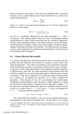


![Simple least-squares methods 235
and setting the derivative to zero gives the well-known normal equations for the
best parameter estimates ¬ :
Ì ¬ Ì (6.18)
which are trivially solved by
¬ ´ Ì µ ½ Ì (6.19)
provided that Ì is invertible. In practice, it is not necessary to invert this
matrix in order to obtain the parameter estimates. In fact, solutions which avoid
this are preferable in terms of speed [102, 209]. However, as shown later, the
matrix ´ Ì µ ½ contains valuable information. A stable method of solution
like LU decomposition [209] should always be used.
In practice, direct solution of the normal equations via (6.19) is not
recommended as problems can arise if the matrix Ì is close to singularity.
Suppose that the right-hand side of equation (6.19) has a small error Æ due to
round-off say, the resulting error in the estimated parameters is given by
Ƭ ´ Ì µ ½ Ì Æ (6.20)
As the elements in the inverted matrix are inversely proportional to the
determinant of Ì , they can be arbitrarily large if Ì is close to
singularity. As a consequence, parameters with arbitrarily large errors can be
obtained. This problem can be avoided by use of more sophisticated techniques.
The near-singularity of the matrix Ì will generally be due to correlations
between its columns (recall that a matrix is singular if two columns are equal),
i.e. correlations between model terms. It is possible to transform the set of
equations (6.19) into a new form in which the columns of the design matrix are
uncorrelated, thus avoiding the problem. Techniques for accomplishing this will
be discussed in Appendix E.
6.3.2 Parameter uncertainty
Because of random errors in the measurements, different samples of data will
contain different noise components and consequently they will lead to slightly
different parameter estimates. The parameter estimates therefore constitute a
random sample from a population of possible estimates; this population being
characterized by a probability distribution. Clearly, it is desirable that the
expected value of this distribution should coincide with the true parameters.
If such a condition holds, the parameter estimator is said to be unbiased and
the necessary conditions for this situation will be discussed in the next section.
Now, given that the unbiased estimates are distributed about the true parameters,
knowledge of the variance of the parameter distribution would provide valuable
Copyright © 2001 IOP Publishing Ltd](https://image.slidesharecdn.com/72268096-non-linearity-in-structural-dynamics-detection-identification-and-modelling-copy-120717010202-phpapp02/85/72268096-non-linearity-in-structural-dynamics-detection-identification-and-modelling-copy-251-320.jpg)
![236 System identification—discrete time
information about the possible scatter in the estimates. This information turns out
to be readily available; the covariance matrix ¦ for the parameters is defined by
¦´ ¬ µ ´ ¬ ¬ µ¡´ ¬ ¬ µÌ (6.21)
where the quantities with carets are the estimates and the expectation is taken
over all possible estimates. The diagonal elements of this matrix, ¾ , are the
variances of the parameter estimates ¬ .
Under the assumption that the estimates are unbiased and therefore
¬ ¬ where ¬ are now the true parameters, then
¦´ ¬ µ ´ ¬ ¬ µ ¡ ´ ¬ ¬ µÌ (6.22)
Now, substituting equation (6.14) containing the true parameters into
equation (6.19) for the estimates, yields
¬ ¬ ·´ Ì µ ½ Ì (6.23)
or, trivially
¬ ¬ ´ Ì µ ½ Ì (6.24)
which can be immediately substituted into (6.22) to give
¦ ´ Ì µ ½ Ì Ì ´ Ì µ ½ (6.25)
Now, it has been assumed that the only variable which changes from
measurement to measurement if the excitation is repeated exactly is . Further,
if is independent of , i.e. independent of Ü and Ý etc, then in this
particular case
¦ ´ Ì µ ½ Ì Ì ´ Ì µ ½ (6.26)
In order to proceed further, more assumptions must be made. First assume
that the noise process is zero-mean, i.e. ¼. In this case the
expectation in equation (6.26) is the covariance matrix of the noise process, i.e.
Ì (6.27)
and further assume that
¾Æ (6.28)
where ¾ is the variance of the residual sequence and Æ is the Kronecker delta.
Under this condition, the expression (6.26) collapses to
¦ ¾´ Ì µ ½ (6.29)
The standard deviation for each estimated parameter is, therefore,
Õ
´ Ì µ ½ (6.30)
Now, if the parameter distributions are Gaussian, standard theory [17] yields
a 95% confidence interval of ¬ ¦ ½ , i.e. there is a 95% probability that
the true parameters fall within this interval.
Copyright © 2001 IOP Publishing Ltd](https://image.slidesharecdn.com/72268096-non-linearity-in-structural-dynamics-detection-identification-and-modelling-copy-120717010202-phpapp02/85/72268096-non-linearity-in-structural-dynamics-detection-identification-and-modelling-copy-252-320.jpg)


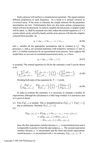

![242 System identification—discrete time
MA model in the terminology introduced in chapter 1. The general noise model
of this type takes the form
Ò
(6.52)
¼
A more compact model can sometimes be obtained by assuming the more
general ARMA form
Ò Ò
· (6.53)
½ ¼
So, some remarks are required on the subject of parameter estimation if a
noise model is necessary. First of all a structure for the model must be specified,
then the situation is complicated by the fact that the noise signal is unmeasurable.
In this case, an initial fit is made to the data without a noise model, the model
predicted output is then subtracted from the measured output to give an estimate
of the noise signal. This allows the re-estimation of parameters, including now
the noise model parameters. The procedure—fit model–predict output–estimate
noise signal—is repeated until the parameters converge.
6.5 Recursive least squares
The least-squares algorithm described in the last section assumes that all the data
are available for processing at one time. It is termed the batch or off-line estimator.
In many cases it will be interesting to monitor the progress of a process in order
to see if the parameters of the model change with time. Such a situation is not
uncommon—a rocket burning fuel or a structure undergoing failure will both
display time-varying parameters. In the latter case, monitoring the parameters
could form the basis of a non-destructive damage evaluation system. It is clear that
some means of tracking time variation could prove valuable. A naive approach
consists of treating the data as a new batch every time a new measurement
becomes available and applying the off-line algorithm. This is computationally
expensive as a matrix inverse is involved and, in some cases, might not be fast
enough to track changes. Fortunately, it is possible to derive an on-line or
recursive version of the least-squares algorithm which does not require a matrix
inverse at each step. The derivation of this algorithm is the subject of this section 5 .
First, assume the general ARX form for the model as given in equation (6.9).
If Ò measurements have already been accumulated; the form of the least-squares
problem is
Ò Ò ¬ · Ò (6.54)
The derivation can be expressed in terms of the so-called matrix inversion lemma as discussed in
[168]. However, the derivation presented here is considered more instructive, it follows an argument
presented in [30].
Copyright © 2001 IOP Publishing Ltd](https://image.slidesharecdn.com/72268096-non-linearity-in-structural-dynamics-detection-identification-and-modelling-copy-120717010202-phpapp02/85/72268096-non-linearity-in-structural-dynamics-detection-identification-and-modelling-copy-258-320.jpg)


![Recursive least squares 245
yn
a1 b1
a2 b2
yn-1 yn-2 xn-1 xn-2
Figure 6.2. An ARX system considered as a linear neural network.
this algorithm as it stands. The iterative procedure is actually obtained directly
from (6.19), and after Æ iterations the resulting parameters are identical to
those which would be obtained from the off-line estimate using the Æ sets of
measurements. The reason for this is that the recursive procedure remembers all
past measurements and weights them equally. Fortunately, a simple modification
exists which allows past data to be weighted with a factor which decays
exponentially with time, i.e. the objective function for minimization is
ÂÒ·½ ÂÒ · ´ÝÒ·½ Ì·½ ¬ µ¾
Ò (6.70)
where is a forgetting factor, i.e. if ½, past data are weighted out.
The required update formulae are [167]
È ·½
à ·½
·½ Ì È
(6.71)
· ·½
½
È ·½ ´½ Ã ·½ Ì µ È
·½ (6.72)
with (6.68) unchanged. In this formulation the parameter estimates can keep
track of variation in the true system parameters. The smaller is, the faster
the procedure can respond to changes. However, if is too small the estimates
become very susceptible to spurious variations due to measurement noise. A value
for in the range 0.9–0.999 is usually adopted.
When the measurements are noisy, the RLS method is well known to give
biased estimates and more sophisticated approaches are needed. The double least-
squares (DLS) method [67] averages the estimates of two approaches, one that
tends to give a positive damping bias and a second that usually gives a negative
damping bias. The DLS technique has been shown to work well on simulated
structural models based on the ARX [67]. The on-line formulation is very similar
Copyright © 2001 IOP Publishing Ltd](https://image.slidesharecdn.com/72268096-non-linearity-in-structural-dynamics-detection-identification-and-modelling-copy-120717010202-phpapp02/85/72268096-non-linearity-in-structural-dynamics-detection-identification-and-modelling-copy-261-320.jpg)

![Analysis of a time-varying linear system 247
Figure 6.3. Experimental arrangement for a time-varying cantilever experiment.
was allowed to ‘warm-up’. (Note also that the integration routine removes a
little data from the beginning and end of the record.) Another slight problem
was caused by the fact that it was impossible to release the water without
communicating some impulse to the system.
The model structure (6.9) was used as it is appropriate to a SDOF system. In
general the minimal model needed for a Æ degree-of-freedom system is
¾Æ ¾Æ ½
Ý Ý · Ü (6.76)
½ ½
and this is minimal because it assumes the simplest discretization rule for the
derivatives.
A minor problem with discrete-time system identification for the structural
dynamicist is that the model coefficients have no physical interpretation.
However, although it is difficult to convert the parameters to masses, dampings
and stiffnesses, it is relatively straightforward to obtain frequencies and damping
ratios [152]. One proceeds via the characteristic polynomial
¾Æ
´Ôµ ½ Ô¾Æ (6.77)
½
whose roots (the poles of the model) are given by
Ô ÜÔ¡Ø´ Ò ¦ µ (6.78)
Copyright © 2001 IOP Publishing Ltd](https://image.slidesharecdn.com/72268096-non-linearity-in-structural-dynamics-detection-identification-and-modelling-copy-120717010202-phpapp02/85/72268096-non-linearity-in-structural-dynamics-detection-identification-and-modelling-copy-263-320.jpg)

![Practical matters 249
Figure 6.5. Identified parameters from the experimental cantilever beam without water,
½: (a) frequency; (b) damping ratio.
In the next chapter, methods for directly extracting physical parameters are
presented.
6.7 Practical matters
The last section raised certain questions about the practice of experimentation for
system identification. This section makes a number of related observations.
6.7.1 Choice of input signal
In the system identification literature, it is usually said that an input signal must
be persistently exciting if it is to be of use for system identification. There are
numerous technical definitions of this term of varying usefulness [231]. Roughly
Copyright © 2001 IOP Publishing Ltd](https://image.slidesharecdn.com/72268096-non-linearity-in-structural-dynamics-detection-identification-and-modelling-copy-120717010202-phpapp02/85/72268096-non-linearity-in-structural-dynamics-detection-identification-and-modelling-copy-265-320.jpg)

![Practical matters 251
Now, it is a trivial fact that
´Ñ ¾ · «µ × Ò´ ص · Ó×´ ص · ´ «µ × Ò´ ص × Ò´ Ø µ
(6.80)
is identically satisfied with « arbitrary. Therefore, the system
«
Ñ ¾ Ý· Ý·´ «µÝ × Ò´ Ø µ (6.81)
explains the input–output process just as well as the true (6.2). This is simply a
manifestation of linear dependence, i.e. there is the relation
Ý ¾Ý (6.82)
and this will translate into discrete time as
Ý · ´ ¾ ¾µÝ ½ · Ý ¾ ¼ (6.83)
So the sine-wave is unsuitable for linear system identification. If one consults
[231], one finds that the sine-wave is only persistently exciting of the very lowest
order. Matters are improved by taking a sum of Æ sinusoids
Æ
ܴص × Ò´ ص (6.84)
½
and it is a simple matter to show that the presence of even two sinusoids is
sufficient to break the linear dependence (6.82) (although the two frequencies
should be reasonably separated).
In the case of a nonlinear system, the presence of harmonics is sufficient to
break linear dependence even if a single sinusoid is used, i.e.
ݴص ½ × Ò´ ص · ¿ × Ò´¿ ص · ¡ ¡ ¡ (6.85)
ݴص ¾ ½ × Ò´ ص · ¾ ¿ × Ò´¿ ص · ¡ ¡ ¡ (6.86)
However, the input is still sub-optimal [271B].
6.7.2 Choice of output signal
This constitutes a real choice for structural dynamicists as the availability of the
appropriate sensors means that it is possible to obtain displacement, velocity or
acceleration data.
For a linear system, the choice is almost arbitrary, differentiation of (6.2)
yields the equations of motion for the linear SDOF system if velocity or
acceleration is observed.
ÑÚ · Ú · Ú Ü´Øµ (6.87)
Copyright © 2001 IOP Publishing Ltd](https://image.slidesharecdn.com/72268096-non-linearity-in-structural-dynamics-detection-identification-and-modelling-copy-120717010202-phpapp02/85/72268096-non-linearity-in-structural-dynamics-detection-identification-and-modelling-copy-267-320.jpg)
![252 System identification—discrete time
and
Ñ · · ܴص (6.88)
which result in discrete-time forms
Ú ½ Ú ½ · ¾ Ú ¾ ½ Ü ½ · ¾ Ü ¾ (6.89)
and
½ ½ · ¾ ¾ ¼ Ü · ½ Ü ½ · ¾ Ü ¾ (6.90)
which are a little more complicated than (6.7). The only slight difference is a few
more lagged Ü terms and the present of the current input Ü in the acceleration
form. Note also that the coefficients of the AR part are unchanged. This might be
expected as they specify the characteristic polynomial from which the frequencies
and dampings are obtained.
If the system is nonlinear, i.e. Duffing’s system (anticipating (6.94)), the
situation is different. On the one hand, the harmonics of the signal are weighted
higher in the velocity and even more so in the acceleration, and this might suggest
that these forms are better for fitting nonlinear terms. On the other hand the
equations of motion become considerably more complex. For the velocity state,
the Duffing system has the equation
Ø Ø ¾ Ø ¿
ÑÚ · Ú · · ½ Ú´ µ · ¾ Ú´ µ · ¿ Ú´ µ ܴص
(6.91)
or
Ø Ø
ÑÚ · Ú · ½ Ú · Ú Ú´ µ ¾ ¾·¿ ¿ Ú´ µ ܴص (6.92)
either form being considerably more complicated than (6.94). The equation of
motion for the acceleration data is more complicated still. It is known that it
is difficult to fit time-series models with polynomial terms to force–velocity or
force–acceleration data from a Duffing oscillator system [58].
In the case of the Duffing system, the simplest structure is obtained if all
three states are measured and used in the modelling. This is the situation with the
direct parameter estimation approach discussed in the next chapter.
6.7.3 Comments on sampling
The choice of sampling frequency is inseparable from the choice of input
bandwidth. Shannon’s criterion [129] demands that the sampling frequency
should be higher than twice the frequency of interest to avoid aliasing. In the
case of a linear system, this means twice the highest frequency in the input. In
the case of a nonlinear system, the frequency should also capture properly the
appropriate number of harmonics. Having said this, the effect of aliasing on
system identification for discrete-time systems is not clear.
Copyright © 2001 IOP Publishing Ltd](https://image.slidesharecdn.com/72268096-non-linearity-in-structural-dynamics-detection-identification-and-modelling-copy-120717010202-phpapp02/85/72268096-non-linearity-in-structural-dynamics-detection-identification-and-modelling-copy-268-320.jpg)
![Practical matters 253
Surprisingly, it is also possible to oversample for the purposes of system
identification. Ljung [167] summarizes his discussion on over-sampling as
follows.
¯ ‘Very fast sampling leads to numerical problems, model fits in high-
frequency bands, and poor returns for hard work.’
¯ ‘As the sampling interval increases over the natural time constants of the
system, the variance (of parameter estimates) increases drastically.’ (In fact,
he shows analytically for a simple example that the parameter variance tends
to infinity as the sampling interval ¡Ø tends to zero [167] p 378.)
¯ ‘Optimal choices of ¡Ø for a fixed number of samples will lie in the range
of the time constants of the system. These are, however, not known, and
overestimating them may lead to very bad results.’
Comprehensive treatments of the problem can also be found in [119] and
[288]. A useful recent reference is [146].
It is shown in [277] that there is a very simple explanation for oversampling.
As the sampling frequency increases, there comes a point where the estimator
can do better by establishing a simple linear interpolation than it can by finding
the true model. An approximate upper bound for the over-sampling frequency is
given by
× ¿¾ ¾ Ñ Ü
½ ½
(6.93)
for high signal-to-noise ratios .
(This result can only be regarded as an existence result due to the fact that
the signal-to-noise ratio would not be known in practice.)
6.7.4 The importance of scaling
In the previous discussion of normal equations, it was mentioned that the
conditioning and invertibility of the information matrix Ì is critical. The
object of this short section is to show how scaling of the data is essential to
optimize the condition of this matrix. The discussion will be by example, data are
simulated from a linear SDOF system (6.2) and a discrete-time Duffing oscillator
(6.95).
It is assumed that the model structure (6.7) is appropriate to linear SDOF
data, so the design matrix would take the form given in (6.13). A system with
a linear stiffness of ½¼ was taken for the example, and this meant that
an input force ܴص with rms ¼ ¾¾, generated a displacement response with rms
¢ ½¼ . There is consequently a large mismatch between the scale of the
first two columns of and the third. This mismatch is amplified when is
effectively squared to form the information matrix
¼ ½
¼ ½¼ ¢ ½¼ ¼¿ ¢ ½¼ ¼½ ¢ ½¼ ¾
¼ ¼ ¢ ½¼ ¼¿ ¢ ½¼ ¼½ ¢ ½¼ ¾
¼ ½½ ¼½ ¢ ½¼ ¾ ¼¿ ¢ ½¼¿
Copyright © 2001 IOP Publishing Ltd](https://image.slidesharecdn.com/72268096-non-linearity-in-structural-dynamics-detection-identification-and-modelling-copy-120717010202-phpapp02/85/72268096-non-linearity-in-structural-dynamics-detection-identification-and-modelling-copy-269-320.jpg)

![NARMAX modelling 255
and the check matrix was
¼
½ ¼¼¼ ¼ ¼¼¼ ¼ ¼¼¼ ¼ ¼¼¼ ½
¼ ¼¼¼ ½ ¼¼¼ ¼ ¼¼¼ ¼ ¼¼¼
¼ ¼¼¼ ¼ ¼¼¼ ½ ¼¼¼ ¼ ¼¼¼
¼ ¼¼¼ ¼ ¼¼¼ ¼ ¼¼¼ ½ ¼¼¼
as required. This example shows that without appropriate scaling, the normal
equations approach can fail due to condition problems. Scaling also produces
marked improvements if the other least-squares techniques are used.
6.8 NARMAX modelling
All the discussion so far has concerned linear systems. This does not constitute
a restriction. The models described are all linear in the parameters so linear
least-squares methods suffice. The models can be extended to nonlinear systems
without changing the algorithm as will be seen. Arguably the most versatile
approach to nonlinear discrete-time systems is the NARMAX (nonlinear auto-
regressive moving average with eXogenous inputs) methodology which has been
developed over a considerable period of time by S A Billings and numerous co-
workers. An enormous body of work has been produced; only the most basic
overview can be given here. The reader is referred to the original references for
more detailed discussions, notably [59, 60, 149, 161, 162].
The extension of the previous discussions to nonlinear systems is
straightforward. Consider the Duffing oscillator represented by
ÑÝ · Ý · Ý · ¿ Ý ¿ ܴص (6.94)
i.e. the linear system of (6.2) augmented by a cubic term. Assuming the simplest
prescriptions for approximating the derivatives as before, one obtains, in discrete
time,
Ý ½ Ý ½ · ¾ Ý ¾ · ½ Ü ½ · Ý¿ ½ (6.95)
where ½ , ¾ and ½ are unchanged from (6.7) and
¡Ø¾ ¿
(6.96)
Ñ
The model (6.95) is now termed a NARX (nonlinear ARX) model. The
regression function Ý ´Ý ½ Ý ¾ Ü ½ µ is now nonlinear; it contains a
cubic term. However, the model is still linear in the parameters which have to
be estimated, so all of the methods previously discussed still apply.
If all terms of order three or less were included in the model structure,
i.e. ´Ý ¾ µ¾ Ü ½ etc a much more general model would be obtained (these more
complicated terms often arise, particularly if nonlinear damping is present):
Ý ´¿µ ´Ý ½ Ý ¾ Ü ½ µ (6.97)
Copyright © 2001 IOP Publishing Ltd](https://image.slidesharecdn.com/72268096-non-linearity-in-structural-dynamics-detection-identification-and-modelling-copy-120717010202-phpapp02/85/72268096-non-linearity-in-structural-dynamics-detection-identification-and-modelling-copy-271-320.jpg)
![256 System identification—discrete time
(the superscript denotes the highest-order product terms) which would be
sufficiently general to represent the behaviour of any dynamical systems with
nonlinearities up to third order, i.e. containing terms of the form Ý ¿ , Ý ¾ Ý etc.
The most general polynomial NARX model (including products of order
ÒÔ ) is denoted by
Ý ´ÒÔµ ´Ý ½ Ý ÒÝ Ü ½ Ü ÒÜ µ (6.98)
It has been proved in the original papers by Leontaritis and Billings
[161, 162], that under very mild assumptions, any input–output process has a
representation by a model of the form (6.98). If the system nonlinearities are
polynomial in nature, this model will represent the system well for all levels
of excitation. If the system nonlinearities are not polynomial, they can be
approximated arbitrarily accurately by polynomials over a given range of their
arguments (Weierstrass approximation theorem [228]). This means that the
system can be accurately modelled by taking the order Ò Ô high enough. However,
the model would be input-sensitive as the polynomial approximation required
would depend on the data. This problem can be removed by including non-
polynomial terms in the NARX model as described in [33].
For example, consider the equation of motion of the forced simple pendulum
Ý · × ÒÝ Ü´Øµ (6.99)
or, in discrete time,
Ý ½ Ý ½ · ¾ Ý ¾ · ½ Ü ½ · × Ò´Ý ½ µ (6.100)
The most compact model of this system will be obtained by including a basis
term × Ò´Ý ½ µ rather than approximating by a polynomial in Ý ½ .
The preceding analysis unrealistically assumes that the measured data are
free of noise—this condition is relaxed in the following discussion. However, as
before, it is assumed that the noise signal ´Øµ is additive on the output signal
ݴص. This constituted no restriction when the system was assumed to be linear
but is generally invalid for a nonlinear system. As shown later, if the system is
nonlinear the noise process can be very complex; multiplicative noise terms with
the input and output are not uncommon, but can be easily accommodated by the
algorithms described earlier and in much more detail in [161, 162, 149, 60].
Under the previous assumption, the measured output has the form
ݴص Ý ´Øµ · ´Øµ (6.101)
where Ý ´Øµ is again the ‘clean’ output from the system. If the underlying system
is the Duffing oscillator of equation (6.94), the equation satisfied by the measured
data is now
ÑÝ · Ý · Ý · ¿ Ý¿ Ñ ¿ ´ ¿ · ¿Ý¾ · ¿Ý ¾ ܴص (6.102)
Copyright © 2001 IOP Publishing Ltd](https://image.slidesharecdn.com/72268096-non-linearity-in-structural-dynamics-detection-identification-and-modelling-copy-120717010202-phpapp02/85/72268096-non-linearity-in-structural-dynamics-detection-identification-and-modelling-copy-272-320.jpg)
![Model validity 257
and the corresponding discrete-time equation will contain terms of the form
½ , ¾ , ½ ݾ ½ etc. Note that even simple additive noise on the output
introduces cross-product terms if the system is nonlinear. Although these terms
all correspond to unmeasurable states they must be included in the model. If they
are ignored the parameter estimates will generally be biased. The system model
(6.98) is therefore extended again by the addition of the noise model and takes the
form
Ý ´¿µ ´Ý ½ Ý ¾ Ü ¾ ½ ¾ µ · (6.103)
The term ‘moving-average’ referring to the noise model should now be
understood as a possibly nonlinear regression on past values of the noise. If a
general regression on a fictitious uncorrelated noise process ´Øµ is incorporated,
one obtains the final general form
Ý ´ÒÔµ ´Ý ½ Ý ÒÝ Ü ½ Ü ÒÜ ½ Ò µ · (6.104)
This type of model is the generic NARMAX model.
A completely parallel theory has been developed for the more difficult
case of time-series analysis where only measured outputs are available for the
formulation of a model; this is documented in [244].
The structure detection can be carried out using the significance statistic of
the NARMAX model—the ERR statistic (E.32)—in essentially two ways:
Forward selection. The model begins with no terms. All one-term models are
fitted and the term which gives the greatest ERR, i.e. the term which accounts
for the most signal variance is retained. The process is iterated, at each step
including the term with greatest ERR and is continued until an acceptable
model error is obtained.
Backward selection. The model begins with all terms and at the first step, the
term with smallest ERR is deleted. Again the process is iterated until the
accepted error is obtained.
Forward selection is usually implemented as it requires fitting smaller
models. To see how advantageous this might be, note that the number of terms in
a generic NARMAX model is roughly
ÒÔ
´ÒÝ · ÒÜ · Ò µÒÔ
(6.105)
¼ ÒÔ
with the various lags etc as previously defined.
6.9 Model validity
Having obtained a NARMAX model for a system, the next stage in the
identification procedure is to determine if the structure is correct and the
Copyright © 2001 IOP Publishing Ltd](https://image.slidesharecdn.com/72268096-non-linearity-in-structural-dynamics-detection-identification-and-modelling-copy-120717010202-phpapp02/85/72268096-non-linearity-in-structural-dynamics-detection-identification-and-modelling-copy-273-320.jpg)
![258 System identification—discrete time
parameter estimates are unbiased. It is important to know if the model has
successfully captured the system dynamics so that it will provide good predictions
of the system output for different input excitations, or if it has simply fitted the
model to the data; in which case it will be of little use since it will only be
applicable to one data set. Three basic tests of the validity of a model have been
established [29], they are now described in increasing order of stringency. In
the following, Ý denotes a measured output while Ý denotes an output value
predicted by the model.
6.9.1 One-step-ahead predictions
Given the NARMAX representation of a system
Ý ´ÒÔ µ ´Ý ½ Ý ÒÝ Ü ½ Ü ÒÜ ½ Ò µ · (6.106)
the one-step-ahead (OSA) prediction of Ý is made using measured values for
all past inputs and outputs. Estimates of the residuals are obtained from the
expression Ý Ý , i.e.
Ý ´ÒÔ µ ´Ý ½ Ý ÒÝ Ü ½ Ü ÒÜ ½ Ò µ (6.107)
The OSA series can then be compared to the measured outputs. Good
agreement is clearly a necessary condition for model validity.
In order to have an objective measure of the goodness of fit, the normalized
mean-square error (MSE) is introduced; the definition is
½¼¼ Æ
MSE´Ý µ ¾ ´Ý
Æ Ý ½
Ý µ¾ (6.108)
where the caret denotes an estimated quantity. This MSE has the following useful
property; if the mean of the output signal Ý is used as the model, i.e. Ý Ý for
all , the MSE is 100.0, i.e.
½¼¼ Æ ½¼¼
MSE´Ý µ ¾ ´Ý
Æ Ý ½
Ý µ¾ ¾
¾ ¡ Ý ½¼¼ (6.109)
Ý
Experience shows that an MSE of less than 5.0 indicates good agreement
while one of less than 1.0 reflects an excellent fit.
6.9.2 Model predicted output
In this case, the inputs are the only measured quantities used to generate the model
output, i.e.
Ý ´ÒÔ µ ´Ý ½ Ý ÒÝ Ü ½ Ü ÒÜ ¼ ¼µ (6.110)
Copyright © 2001 IOP Publishing Ltd](https://image.slidesharecdn.com/72268096-non-linearity-in-structural-dynamics-detection-identification-and-modelling-copy-120717010202-phpapp02/85/72268096-non-linearity-in-structural-dynamics-detection-identification-and-modelling-copy-274-320.jpg)
![Model validity 259
The zeroes are present because the prediction errors will not generally be
available when one is using the model to predict output. In order to avoid a
misleading transient at the start of the record for Ý, the first Ò Ý values of the
measured output are used to start the recursion. As before, the estimated outputs
must be compared with the measured outputs, with good agreement a necessary
condition for accepting the model. It is clear that this test is stronger than the
previous one; in fact the OSA predictions can be excellent in some cases when the
model-predicted output (MPO) shows complete disagreement with the measured
data.
6.9.3 Correlation tests
These represent the most stringent of the validity checks. The appropriate
reference is [34]. The correlation function ÙÚ ´ µ for two sequences of data Ù
and Ú is defined as usual by
½ Æ
ÙÚ ´Ù Ú · µ ÙÚ·
Æ
(6.111)
½
In practice, normalized estimates of all the previous correlation functions are
obtained using
½ ÈÆ Ù Ú ·
Æ ½
ÙÚ ´ µ ¾ ¾ ½ ¼ (6.112)
´Ù µ ´Ú µ ¾
with a similar expression for ¼. The normalized expression is used because
it allows a simple expression for the 95% confidence interval for a zero result,
Ô
namely ¦½ ´Æ µ. The confidence limits are required because the estimate
of ÙÚ is made only on a finite set of data; as a consequence it will never be truly
zero. The model is therefore considered adequate if the correlation functions
described earlier fall within the 95% confidence limits. These limits are indicated
by a broken line when the correlation functions are shown later.
For a linear system it is shown in [34], that necessary conditions for model
validity are
´ µ Ƽ (6.113)
Ü ´ µ ¼ (6.114)
The first of these conditions is true only if the residual sequence is a white-
noise sequence. It is essentially a test of the adequacy of the noise model whose
job it is to reduce the residuals to white noise. If the noise model is correct,
the system parameters should be free from bias. The second of these conditions
states that the residual signal is uncorrelated with the input sequence Ü , i.e. the
model has completely captured the component of the measured output which is
correlated with the input. Another way of stating this requirement is that the
residuals should be unpredictable from the input.
Copyright © 2001 IOP Publishing Ltd](https://image.slidesharecdn.com/72268096-non-linearity-in-structural-dynamics-detection-identification-and-modelling-copy-120717010202-phpapp02/85/72268096-non-linearity-in-structural-dynamics-detection-identification-and-modelling-copy-275-320.jpg)
![260 System identification—discrete time
In the case of a nonlinear system it is sometimes possible to satisfy these
requirements even if the model is invalid. It is shown in [34] that an exhaustive
test of the fitness of a nonlinear model requires the evaluation of three additional
correlation functions. The extra conditions are
´ ܵ ´ µ ¼ ¼ (6.115)
ܾ¼ ´ µ ¼ (6.116)
ܾ¼ ¾ ´ µ ¼ (6.117)
The prime which accompanies the ܾ indicates that the mean has been
removed.
6.9.4 Chi-squared test
One final utility can be mentioned. If the model fails the validity tests one can
compute a statistic as in [60] for a given term not included in the model to see
if it should be present. The test is specifically developed for nonlinear systems
and is based on chi-squared statistics. A number of values of the statistic for a
specified term are plotted together with the 95% confidence limits. If values of
the statistic fall outside the limits, the term should be included in the model and
it is necessary to re-estimate parameters accordingly. Examples of all the test
procedures described here will be given in the following section.
6.9.5 General remarks
Strict model validation requires that the user have a separate set of testing data
from that used to form the model. This is to make sure that the identification
scheme has learnt the underlying model and not simply captured the features of
the data set. The most rigorous approach demands that the testing data have a
substantially different form from the estimation data. Clearly different amplitudes
can be used. Also, different excitations can be used. For example if the model is
identified from data from Gaussian white-noise excitation, the testing data could
come from PRBS (pseudo-random binary sequence) or chirp.
6.10 Correlation-based indicator functions
Having established the normalized correlation functions in the last section, it is
an opportune moment to mention two simple correlation tests which can signal
nonlinearity by manipulating measured time data. If records of both input Ü and
output Ý are available, it can be shown that the correlation function
ܾ ݼ ´ µ Ü Ý ¼· (6.118)
vanishes for all if and only if the system is linear [35]. The prime signifies that
the mean has been removed from the signal.
Copyright © 2001 IOP Publishing Ltd](https://image.slidesharecdn.com/72268096-non-linearity-in-structural-dynamics-detection-identification-and-modelling-copy-120717010202-phpapp02/85/72268096-non-linearity-in-structural-dynamics-detection-identification-and-modelling-copy-276-320.jpg)
![Analysis of a simulated fluid loading system 261
If only sampled outputs are available, it can be shown that under certain
conditions [31], the correlation function
ݼ ݼ ¾ ´ µ Ý ¼ · ´Ý ¼ µ¾ (6.119)
is zero for all if and only if the system is linear. In practice, these functions
will never be identically zero; however, confidence intervals for a zero result
can be calculated straightforwardly. As an example the correlation functions for
acceleration data from an offset bilinear system at both low and high excitation
are shown in figure 6.7; the broken lines are the 95% confidence limits for a
zero result. The function in figure 6.7(b) indicates that the data from the high
excitation test arise from a nonlinear system. The low excitation test did not
excite the nonlinearity and the corresponding function (figure 6.7(a)) gives a null
result as required.
There are a number of caveats associated with the latter function. It is a
necessary condition that the third-order moments of the input vanish and all even-
order moments exist. This is not too restrictive in practice; the conditions hold
for a sine wave or a Gaussian noise sequence for example. More importantly,
the function (6.119) as it stands only detects even nonlinearity, e.g. quadratic
stiffness. In practice, to identify odd nonlinearity, the input signal should contain
a d.c. offset, i.e. a non-zero mean value. This offsets the output signal and adds
an even component to the nonlinear terms, i.e.
Ý¿ ´Ý · ݵ¿ Ý¿ · ¿Ý¾Ý · ¿Ýݾ · Ý¿ (6.120)
A further restriction on (6.119) is that it cannot detect odd damping
nonlinearity 7, as it is not possible to generate a d.c. offset in the velocity to add an
odd component to the nonlinearity. Figure 6.8 shows the correlation function for
a linear system and a system with Coulomb friction, the function fails to signal
nonlinearity. (Note that the coherence function in the latter case showed a marked
decrease which indicated strong nonlinearity.)
6.11 Analysis of a simulated fluid loading system
In order to demonstrate the concepts described in previous sections, the
techniques are now applied to simulated data from the Morison equation, which
is used to predict forces on offshore structures [192],
´Øµ ½ ÙÙ ·½ ¾ ÑÙ
¾ (6.121)
where ´Øµ is the force per unit axial length, ٴص is the instantaneous flow
velocity, is water density and is diameter; and Ñ are the dimensionless
drag and inertia coefficients. The first problem is to determine an appropriate
The authors would like to thank Dr Steve Gifford for communicating these results to them [112]
and giving permission for their inclusion.
Copyright © 2001 IOP Publishing Ltd](https://image.slidesharecdn.com/72268096-non-linearity-in-structural-dynamics-detection-identification-and-modelling-copy-120717010202-phpapp02/85/72268096-non-linearity-in-structural-dynamics-detection-identification-and-modelling-copy-277-320.jpg)


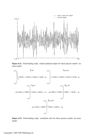
![Analysis of a simulated fluid loading system 267
Figure 6.13. Fluid-loading study: chi-squared tests for linear process model—no noise
model.
model is probably not needed. The values of the exact NARMAX coefficients for
the data were ½ ½ , ¾ ¾ ¿¾ and ¿ ¼ ¼¼ .
In order to demonstrate fully the capabilities of the procedures, a coloured
noise signal was added to the force data. The noise model chosen was
¼ ¾¾¾ ½½½ ½ ¾ · ¿ (6.127)
where was a Gaussian white-noise sequence. The variance of ´Øµ was chosen
in such a way that the overall signal-to-noise ratio would be equal to
5.0. This corresponds to the total signal containing approximately 17% noise.
This is comparatively low, a benchtest study described in [270] showed that the
NARMAX procedures could adequately identify Morison-type systems with the
signal-to-noise ratio as high as unity.
The first attempt to model the data assumed the linear structure
½ Ù · ¾ Ù ½ (6.128)
The resulting parameter estimates were ½ and ¾ ¿½ ½ with
standard deviations ½ ¾ and ¾ ¾. The estimated value of ½ is 7.0
standard deviations away from the true parameter; this indicates bias. The reason
for the overestimate is that the Ù ¿ term which should have been included in the
Copyright © 2001 IOP Publishing Ltd](https://image.slidesharecdn.com/72268096-non-linearity-in-structural-dynamics-detection-identification-and-modelling-copy-120717010202-phpapp02/85/72268096-non-linearity-in-structural-dynamics-detection-identification-and-modelling-copy-283-320.jpg)


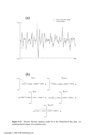

![Analysis of a real fluid loading system 273
Table 6.2. Parameter table for NARMAX model of Christchurch Bay data.
Model term Parameter
½ ¼½ · ¼½
¾ ¼ ½¾ · ¼½
¿ ¼ ¼ ¼½
¼¿ · ¼¼
¼ ¿¾ · ¼¼
¼ ½½½ · ¼¼
Ù ¼ ½½ · ¼¿
Ù ½ ¼ ¿¼¼ · ¼¿
Ù ¾ ¼ ¿¾¿ · ¼¿
Ù ¿ ¼ ½ · ¼¿
Ù ¼ · ¼½
Ù ¼¾ ¿ · ¼¾
¾ ¿ ¼ ½ ¿ ¼¿
¾
¿ ½
¼ ½¿ ¼¿
¼ ¾¿¾ ¼
¾ ½ ¼ ½ ¿ ¼
½ Ù¾ ¼ ¾¾½ · ¼¼
Ù¾ ¼½ · ¼¼
¿ Ù Ù ¼ · ¼¼
¾ Ù¾ ¿ ¼ · ¼¼
½ ¾ Ù
¾ ½ Ù
¼ ¿½ ¼¿
¼ ¾ ¼¿
Ù ¿ Ù¾ ¼ ¿ · ¼¾
Ù Ù¾ ¼½ · ¼¿
Ù ½ Ù¾ ¼ ½ · ¼¿
¿ ¾ ¼ ½¼½ ¼
½ ¾ ¼ ¾¾¾ ¼
¾ ½ ¾ ¿ ¼ ¿ ¼
¾ ½ ¾ ¼ ½¾¼ ¼
6.12 Analysis of a real fluid loading system
In this section the NARMAX model structure is fitted to forces and velocities
measured on the Christchurch Bay Tower which was constructed to test (amongst
other things) fluid loading models in a real directional sea environment. The tower
is shown in figure 6.15 and is described in considerable more detail in [39].
The tower was instrumented with pressure transducers and velocity meters.
The data considered here were measured on the small diameter wave staff
(Morison’s equation is only really appropriate for slender members). Substantial
wave heights were observed in the tests (up to 7 m) and the sea was directional
with a prominent current. The velocities were measured with calibrated perforated
Copyright © 2001 IOP Publishing Ltd](https://image.slidesharecdn.com/72268096-non-linearity-in-structural-dynamics-detection-identification-and-modelling-copy-120717010202-phpapp02/85/72268096-non-linearity-in-structural-dynamics-detection-identification-and-modelling-copy-289-320.jpg)


![Identification using neural networks 277
Figure 6.22. Correlation tests for linear system identification example using a neural
network.
conditions [199]. The MPO and correlation tests are shown in figure 6.18.
Although the validity tests show a great deal of improvement, the MPO appears to
be worse. This is perfectly understandable; one of the effects of correlated noise
(indicated by the function in figure 6.17) is to bias the model coefficients so
that the model fits the data rather than the underlying system. In this case the MPO
is actually accounting for some of the system noise; this is clearly incorrect. When
the noise model is added to reduce the noise to a white sequence, the unbiased
model no longer predicts the noise component and the MPO appears to represent
the data less well. This is one reason why the MSE adopted here makes use of the
residual sequence rather than the prediction errors . In this case, the MSE is
0.75 which shows a marked improvement over the Morison equation. The fact that
the final correlation function in figure 6.18 still indicates problems with the model
can probably be attributed to the time-dependent phase relationship between input
and output described earlier.
6.13 Identification using neural networks
6.13.1 Introduction
The problem of system identification in its most general form is the construction
of the functional Ë which maps the inputs of the system to the outputs. The
problem has been simplified considerably in the discussion so far by assuming
that a linear-in-the-parameters model with an appropriate structure can be used.
Either an a priori structure is assumed or clever structure detection is needed. An
alternative approach would be to construct a complete ‘black-box’ representation
Copyright © 2001 IOP Publishing Ltd](https://image.slidesharecdn.com/72268096-non-linearity-in-structural-dynamics-detection-identification-and-modelling-copy-120717010202-phpapp02/85/72268096-non-linearity-in-structural-dynamics-detection-identification-and-modelling-copy-293-320.jpg)


![280 System identification—discrete time
Figure 6.25. Correlation tests for the linear neural network model of the Duffing oscillator.
system is
Ò ÒÝ ÒÜ ½
Ý ×· Û ØÒ Ú Ý · Ù Ñ Ü Ñ · (6.131)
½ ½ Ñ ¼
or, if a nonlinear output neuron is used,
Ò ÒÝ ÒÜ ½
Ý Ø Ò ×· Û ØÒ Ú Ý · Ù Ñ Ü Ñ · (6.132)
½ ½ Ñ ¼
For the RBF network
Ò ÒÝ ÒÜ ½
Ý ×· Û ÜÔ ¾½ ¾ ´Ý Ú µ¾ · ´Ü Ñ Ù Ñ µ¾
½ ½ Ñ ¼
ÒÝ ÒÜ ½
· Ý · Ü (6.133)
½ ßÞ
¼
from linear connections
where the quantities Ú and Ù Ñ are the hidden node centres and the is the
standard deviation or radius of the Gaussian at hidden node . The first part of
this expression is the standard RBF network.
Some of the earliest examples of the use of neural networks for system
identification and modelling are the work of Chu et al [64] and Narendra and
Parthasarathy [194]. Masri et al [179, 180] are amongst the first structural
dynamicists to exploit the techniques. The latter work is interesting because it
Copyright © 2001 IOP Publishing Ltd](https://image.slidesharecdn.com/72268096-non-linearity-in-structural-dynamics-detection-identification-and-modelling-copy-120717010202-phpapp02/85/72268096-non-linearity-in-structural-dynamics-detection-identification-and-modelling-copy-296-320.jpg)
![Identification using neural networks 281
Figure 6.26. Final neural network state for the nonlinear model of the Duffing oscillator.
demonstrates ‘dynamic neurons’ which are said to increase the utility of the MLP
structure for modelling dynamical systems. The most comprehensive programme
of work to date is that of Billings and co-workers starting with [36] for the MLP
Copyright © 2001 IOP Publishing Ltd](https://image.slidesharecdn.com/72268096-non-linearity-in-structural-dynamics-detection-identification-and-modelling-copy-120717010202-phpapp02/85/72268096-non-linearity-in-structural-dynamics-detection-identification-and-modelling-copy-297-320.jpg)
![282 System identification—discrete time
Figure 6.27. OSA and MPO predictions for the nonlinear neural network model of the
Duffing oscillator.
structure and [62] for the RBF.
The use of the neural network will be illustrated with a couple of case studies,
only the MLP results will be shown.
6.13.2 A linear system
The data consists of 999 pairs of input–output data for a linear dynamical system
with equation of motion
Ý · ¾¼Ý · ½¼ Ý Ü´Øµ (6.134)
where ܴص is a zero-mean Gaussian sequence of rms 10.0. (The data were
obtained using a fourth-order Runge–Kutta routine to step the differential
equation forward in time.) The output data are corrupted by zero-mean Gaussian
white noise. A structure using four lags in both input and output were chosen.
Copyright © 2001 IOP Publishing Ltd](https://image.slidesharecdn.com/72268096-non-linearity-in-structural-dynamics-detection-identification-and-modelling-copy-120717010202-phpapp02/85/72268096-non-linearity-in-structural-dynamics-detection-identification-and-modelling-copy-298-320.jpg)

![284 System identification—discrete time
6.13.3.1 A linear model
It is usual in nonlinear system identification to fit a linear model first. This gives
information about the degree of nonlinearity and also provides guidance on the
appropriate values for the lags Ò Ý and ÒÜ . As this is a single-degree-of-freedom
(SDOF) system like that in the first exercise, one can expect reasonable results
using the same lag values. A linear network was tried first.
The final state of the network is saved after the 20 000 presentations; the
result is given in figure 6.23. The MSEs reported by the procedure are 8.72 for
the OSA and 41.04 for the MPO which are clearly unacceptable. Figures 6.24 and
6.25, respectively, show the predictions and correlation tests.
6.13.3.2 A nonlinear model
This time a nonlinear network but with a linear output neuron was used. Eight
hidden units were used. The final network state is shown in figure 6.26. The rms
error shows a vast improvement on the linear network result (figure 6.23). This
is reflected in the network MSEs which were 0.34 (OSA) and 3.10 (MPO). The
network predictions are given in figure 6.27 and the correlation tests in figure 6.28.
It is shown in [275] that the neural network structures discussed here
can represent a broad range of SDOF nonlinear systems, with continuous or
discontinuous nonlinearities. This is one of the advantages of the neural network
approach to identification; a ‘black box’ is specified which can be surprisingly
versatile. The main disadvantage is that the complex nature of the network
generally forbids an analytical explanation of why training sometimes fails to
converge to an appropriate global minimum. For modelling purposes, it is
unfortunate that the structure detection algorithms which prove so powerful in
the NARMAX approach cannot be implemented, although ‘pruning’ algorithms
are being developed which allow some simplification of the network structures.
The network structure and training schedule must be changed if a different set of
lagged variables is to be used.
Copyright © 2001 IOP Publishing Ltd](https://image.slidesharecdn.com/72268096-non-linearity-in-structural-dynamics-detection-identification-and-modelling-copy-120717010202-phpapp02/85/72268096-non-linearity-in-structural-dynamics-detection-identification-and-modelling-copy-300-320.jpg)

![286 System identification—continuous time
The current chapter is not intended to be a comprehensive review of
continuous-time approaches to system ID. Rather, the evolution of a particular
class of models is described. The curious reader can refer to [152] and [287] for
references to more general literature. The thread followed in this chapter begins
with the identification procedure of Masri and Caughey.
7.2 The Masri–Caughey method for SDOF systems
7.2.1 Basic theory
The simple procedure described in this section allows a direct non-parametric
identification for SDOF nonlinear systems. The only a priori information
required is an estimate of the system mass. The basic procedures described
in this section were introduced by Masri and Caughey [174]; developments
discussed later arise from a parallel approach proposed independently by Crawley
and Aubert [70, 71]; the latter method was referred to by them as ‘force-state
mapping’.
The starting point is the equation of motion as specified by Newton’s second
law
ÑÝ · ´Ý ݵ ܴص (7.1)
where Ñ is the mass (or an effective mass) of the system and ´Ý ݵ is the internal
restoring force which acts to return the absorber to equilibrium when disturbed.
The function can be a quite general function of position Ý ´Øµ and velocity Ý ´Øµ.
In the special case when the system is linear
´Ý ݵ Ý· Ý (7.2)
where and are the damping constant and stiffness respectively. Because is
assumed to be dependent only on Ý and Ý it can be represented by a surface over
the phase plane, i.e. the ´Ý ݵ-plane. A trivial re-arrangement of equation (7.1)
gives
´Ý´Øµ ݴصµ ܴص Ñݴص (7.3)
If the mass Ñ is known and the excitation ܴص and acceleration ݴص are
measured, all the quantities on the right-hand side of this equation are known
and hence so is . As usual, measurement of a time signal entails sampling it at
regularly spaced intervals ¡Ø. (In fact, such is the generality of the method that
regular sampling is not essential; however, if any preprocessing is required for the
measured data, regular sampling is usually required.) If Ø ´ ½µ¡Ø denotes
the th sampling instant, then at Ø , equation (7.3) gives
´Ý Ý µ Ü ÑÝ (7.4)
where Ü Ü´Ø µ and Ý Ý´Ø µ and hence are known at each sampling
instant. If the velocities Ý and displacements Ý are also known (i.e. from direct
Copyright © 2001 IOP Publishing Ltd](https://image.slidesharecdn.com/72268096-non-linearity-in-structural-dynamics-detection-identification-and-modelling-copy-120717010202-phpapp02/85/72268096-non-linearity-in-structural-dynamics-detection-identification-and-modelling-copy-302-320.jpg)
![The Masri–Caughey method for SDOF systems 287
measurement or from numerical integration of the sampled acceleration data), at
each instant ½ Æ a triplet ´Ý Ý µ is specified. The first two values
indicate a point in the phase plane, the third gives the height of the restoring force
surface above that point. Given this scattering of force values above the phase
plane there are a number of methods of interpolating a continuous surface on a
regular grid; the procedures used here are discussed a little later.
Once the surface is obtained, Masri and Caughey [174] construct a
parametric model of the restoring force in the form of a double Chebyshev series;
formally
Ñ Ò
´Ý ݵ Ì ´ÝµÌ ´Ýµ (7.5)
¼ ¼
where Ì ´Ý µ is the Chebyshev polynomial of order . The use of these polynomials
was motivated by a number of factors:
¯ They are orthogonal polynomials. This means that one can estimate
coefficients for a double summation or series of order ´Ñ Òµ and the
truncation of the sum to order ´ µ, where Ñ and Ò is the best
approximation of order ´ µ. This means that one need not re-estimate
coefficients if a lower-order model is acceptable. This is not the case for
simple polynomial models. Similarly, if the model needs to be extended, the
coefficients for the lower-order model will still stand.
¯ The estimation method for the coefficients used by Masri and Caughey
required the evaluation of a number of integrals. In the case of the Chebyshev
expansion, a change of variables exists which makes the numerical integrals
fairly straightforward. This is shown later.
¯ In the family of polynomial approximations to a given function over a
given interval, there will be one which has the smallest maximum deviation
from that function over the interval. This approximating polynomial—the
minimax polynomial has so far eluded discovery. However, one of the nice
properties of the Chebyshev expansion is that it is very closely related to
the required minimax expansion. The reason for this is that the error in the
Chebyshev expansion on a given interval oscillates between almost equal
upper and lower bounds. This property is sometimes referred to as the equal-
ripple property.
Although more convenient approaches are now available which make use of
ordinary polynomial expansions, the Masri–Caughey technique is still sometimes
used for MDOF systems, so the estimation procedure for the Chebyshev series
will be given. The various properties of Chebyshev polynomials used in this
study are collected together in appendix H. A comprehensive reference can be
found in [103]. A number of useful numerical routines relating to Chebyshev
approximation can be found in [209].
The first problem encountered in fitting a model of the form (7.5) relates
to the overall scale of the data Ý and Ý. In order to obtain the coefficients ,
Copyright © 2001 IOP Publishing Ltd](https://image.slidesharecdn.com/72268096-non-linearity-in-structural-dynamics-detection-identification-and-modelling-copy-120717010202-phpapp02/85/72268096-non-linearity-in-structural-dynamics-detection-identification-and-modelling-copy-303-320.jpg)

![The Masri–Caughey method for SDOF systems 289
and
´Ù Úµ ´ ½ ´Ùµ ½ ´Úµµ (7.14)
Following a change of coordinates
Ó× ½ ´Ùµ
Ó× ½ ´Úµ (7.15)
the integral (7.13) becomes
Ó×´ µ Ó×´ µ ´ Ó×´ µ Ó×´ µµ (7.16)
¼ ¼
and the troublesome singular functions Û´Ùµ and Û´Ú µ have been removed. The
simplest approach to evaluating this integral is to use a rectangle rule. The -
range ´¼ µ is divided into Ò intervals of length ¡ Ò and the -range
into Ò intervals of length ¡ Ò and the integral is approximated by the
summation
Ò Ò
¡ ¡ Ó×´ µ Ó×´ Ð µ ´ Ó×´ µ Ó×´ Ð µµ (7.17)
½Ð ½
where ´ ½µ¡ and Ð ´Ð ½µ¡ .
At this point, the question of interpolation is raised again. The values of
the force function on a regular grid in the ´Ý Ý µ-plane must be transformed
into values of the function on a regular grid in the ´ µ. This matter will be
discussed shortly.
Once the coefficients have been obtained, the model for the restoring
force is established. To recap
Ñ Ò
´Ý Ý µ Ì ´ ´ÝµµÌ ´ ´Ýµµ (7.18)
¼ ¼
and this is valid on the rectangle Ý Ñ Ò ÝÑ Ü ¢ ÝÑ Ò ÝÑ Ü . As long as the
true form of the restoring force ´Ý Ý µ is multinomial and the force ܴص driving
the system excites the highest-order terms in , the approximation will be valid
throughout the phase plane. If either of these conditions do not hold, the model
will only be valid on the rectangle containing the sample data. If the force ܴص
has not excited the system adequately, the model is input-dependent and may well
lose its predictive power if radically different inputs are used to excite the system.
There is a class of systems for which the restoring force method cannot be
used in the simple form described here, i.e. systems with memory or hysteretic
systems. In this case, the internal force does not depend entirely on the
instantaneous position of the system in the phase plane. As an illustration,
consider the Bouc–Wen model [263]
ÑÝ · ´Ý ݵ · Þ Ü´Øµ (7.19)
Þ « Ý Þ ¡ Þ Ò ½ ¬ Ý Þ Ò · Ý (7.20)
Copyright © 2001 IOP Publishing Ltd](https://image.slidesharecdn.com/72268096-non-linearity-in-structural-dynamics-detection-identification-and-modelling-copy-120717010202-phpapp02/85/72268096-non-linearity-in-structural-dynamics-detection-identification-and-modelling-copy-305-320.jpg)
![290 System identification—continuous time
which can represent a broad range of hysteresis characteristics. The restoring
force surface would fail here because the internal force is a function of Ý , Ý and Þ ;
this means that the force surface over ´Ý Ý µ would appear to be multi-valued. A
smooth surface can be obtained by exciting the system at a single frequency over a
range of amplitudes; however, the surfaces would be different for each frequency.
Extensions of the method to cover hysteretic systems have been devised [27, 169];
models of the type
´ ݵ (7.21)
are obtained which also admit a representation as a surface over the ´ Ý µ plane.
A parametric approach to modelling hysteretic systems was pursued in [285]
where a Bouc–Wen model (7.20) was fitted to measured data; this approach is
complicated by the fact that the model (7.20) is nonlinear in the parameters and a
discussion is postponed until section 7.6 of this chapter.
7.2.2 Interpolation procedures
The problem of interpolating a continuous surface from values specified on
a regular grid is well-known and documented [209]. In this case it is a
straightforward matter to obtain an interpolated value or interpolant which is
many times differentiable. The restoring force data are required on a regular
grid in order to facilitate plotting of the surface. Unfortunately, the data used
to construct a restoring force surface will generally be randomly or irregularly
placed in the phase plane and this makes the interpolation problem considerably
more difficult. A number of approaches are discussed in [182] and [160]. One
method in particular, the natural neighbour method of Sibson [225], is attractive
as it can produce a continuous and differentiable interpolant. The workings of the
methods are rather complicated and involve the construction of a triangulation of
the phase plane, the reader is referred to [225] for details. The software TILE4
[226] was used throughout this study in order to construct the Masri–Caughey
restoring force surfaces.
The advantage of having a higher-order differentiable surface is as follows.
The continuous or ¼ interpolant essentially assumes linear variations in the
interpolated function between the data points, i.e. the interpolant is exact only
for a linear restoring force surface:
´Ý ݵ « · ¬Ý · Ý (7.22)
As a consequence, it can only grow linearly in regions where there are very little
data. As the functions of interest here are nonlinear, this is a disadvantage. The
undesirable effects of this will be shown by example later.
The surfaces produced by natural neighbour interpolation, can be continuous
or differentiable (designated ½ ). Such functions are generally specified by
Copyright © 2001 IOP Publishing Ltd](https://image.slidesharecdn.com/72268096-non-linearity-in-structural-dynamics-detection-identification-and-modelling-copy-120717010202-phpapp02/85/72268096-non-linearity-in-structural-dynamics-detection-identification-and-modelling-copy-306-320.jpg)
![The Masri–Caughey method for SDOF systems 291
quadratic functions 1
´Ý Ý µ « · ¬Ý · Ý · ¯Ý¾ · ÝÝ · ݾ (7.23)
The natural neighbour method is used to solve the first interpolation problem
in the Masri–Caughey approach. The second interpolation is concerned with
going from a regular grid in the phase plane to a regular grid in the ´ µ-
plane. The natural neighbour method could be used again, but it is rather
computationally expensive and as long as a reasonably fine mesh is used, simpler
methods suffice. Probably the simplest is the ¼ bilinear interpolation [209].
If arrays of values Ý , ½ Æ and Ý , ½ Å specify the
locations of the grid points and an array holds the corresponding values of
the force function, the bilinear interpolant at a general point ´Ý ݵ, is obtained as
follows.
(1) Identify the grid-square containing the point ´Ý ݵ, i.e. find ´Ñ Òµ such that
ÝÑ Ý ÝÑ·½
ÝÒ Ý ÝÒ·½ (7.24)
(2) Define
½ ÑÒ
¾ Ñ·½ Ò
¿ Ñ·½ Ò·½
Ñ Ò·½ (7.25)
and
Ø ´Ý ÝÑ µ ´ÝÑ·½ Ýѵ
Ù ´Ý ÝÒµ ´ÝÒ·½ ÝÒ µ (7.26)
(3) Evaluate the interpolant:
´Ý Ý µ ´½ ص´½ Ùµ ½ · Ø´½ Ùµ ¾ · ØÙ ¿ · ´½ ص٠(7.27)
All the machinery required for the basic Masri–Caughey procedure is now
in place and the method can be illustrated on a number of simple systems.
½ In fact, the natural neighbour method is exact for a slightly more restricted class of functions,
namely the spherical quadratics:
´Ý ݵ « · ¬Ý · Ý · ݾ · ݾ
Copyright © 2001 IOP Publishing Ltd](https://image.slidesharecdn.com/72268096-non-linearity-in-structural-dynamics-detection-identification-and-modelling-copy-120717010202-phpapp02/85/72268096-non-linearity-in-structural-dynamics-detection-identification-and-modelling-copy-307-320.jpg)
![292 System identification—continuous time
7.2.3 Some examples
The Masri–Caughey procedure is demonstrated in this section on a number of
computer-simulated SDOF systems. In each case, a fourth-order Runge–Kutta
scheme [209], is used to integrate the equations of motion. Where the excitation
is random, it is generated by filtering a Gaussian white-noise sequence onto the
range 0–200 Hz. The sampling frequency is 1000 Hz (except for the Van der
Pol oscillator). The simulations provide a useful medium for discussing problems
with the procedure and how they can be overcome.
7.2.3.1 A linear system
The first illustration concerns a linear system with equation of motion:
Ý · ¼Ý · ½¼ Ý Ü´Øµ (7.28)
The system was excited with a random excitation with rms 1.0 and 10 000
points of data were collected. The distribution of the points in the phase plane
is shown in figure 7.1. This figure shows the first problem associated with the
method. Not only are the points randomly distributed as discussed earlier, they
Velocity
Displacement
Figure 7.1. Distribution of points in the phase plane for a randomly excited linear system.
Copyright © 2001 IOP Publishing Ltd](https://image.slidesharecdn.com/72268096-non-linearity-in-structural-dynamics-detection-identification-and-modelling-copy-120717010202-phpapp02/85/72268096-non-linearity-in-structural-dynamics-detection-identification-and-modelling-copy-308-320.jpg)


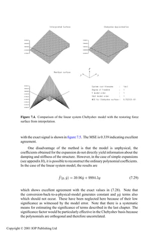


![The Masri–Caughey method for SDOF systems 303
Displacement (m)
Time (sample points)
Figure 7.12. Comparison of the measured Van der Pol oscillator (vdpo) response with
predictions from the Chebyshev model, a later part of the record.
approximation to dry friction is to add a damping term of the form × Ò´Ý µ 2 . To
illustrate the analysis for such systems, data were simulated from an oscillator
with equation of motion
Ý · ¾¼Ý · ½¼ × Ò´Ýµ · ½¼ Ý Ü´Øµ (7.32)
in more or less the same fashion as before. When the ½ restoring force
surface was computed, the result was as shown in figure 7.15; a number of
spikes are visible. These artifacts are the result of the estimation of gradients
for the interpolation. Two points on either side of the discontinuity can yield
an arbitrarily high estimated gradient depending on their proximity. When the
gradient terms (first order in the Taylor expansion) are added to the force estimate,
the interpolant can be seriously in error. The way around the problem is to use
a ¼ interpolant which does not need gradient information. The lower-order
surface for the same data is shown in figure 7.16 and the spikes are absent. If
one is concerned about lack of accuracy in regions of low data density, a hybrid
¾ Friction is actually a lot more complicated than this. A brief but good review of real friction forces
can be found in [183]. This paper is also interesting for proposing a friction model where the force
depends on the acceleration as well as the velocity. Because there are three independent states in such
a model, it cannot be visualized using RFS methods.
Copyright © 2001 IOP Publishing Ltd](https://image.slidesharecdn.com/72268096-non-linearity-in-structural-dynamics-detection-identification-and-modelling-copy-120717010202-phpapp02/85/72268096-non-linearity-in-structural-dynamics-detection-identification-and-modelling-copy-319-320.jpg)


![The Masri–Caughey method for MDOF systems 307
F
y y
Figure 7.16. The identified restoring force surface for data from a Coulomb friction
system: ¼ interpolation.
underlying linear system) will nonetheless yield a worthwhile simplification.
Equation (7.33) becomes
Å Ù · ´Ù Ùµ Դص (7.37)
where Ì . As before, the method assumes that the Ý , Ý and Ý
data are available. However, in the MDOF case, estimates of the mass matrix Å
and modal matrix are clearly needed. For the moment assume that this is the
case; modal analysis at low excitation can provide and there are numerous,
well-documented means of estimating Ñ [11]. The restoring force vector is
obtained from
Ô Å Ù Ì´ Ü Ñ Ý µ (7.38)
Copyright © 2001 IOP Publishing Ltd](https://image.slidesharecdn.com/72268096-non-linearity-in-structural-dynamics-detection-identification-and-modelling-copy-120717010202-phpapp02/85/72268096-non-linearity-in-structural-dynamics-detection-identification-and-modelling-copy-323-320.jpg)

![The Masri–Caughey method for MDOF systems 309
Displacement (m)
Time (sample points)
Figure 7.18. Comparison of the measured Coulomb friction system response with
predictions from the Chebyshev model.
as Ù« Ù¬ . To include the effects of modal coupling due to the nonlinearity, terms
such as Ù« Ù¬ are needed with . Further, if the nonlinearity is in the damping,
the model will need terms of the form Ù « Ù¬ . Finally, consideration of the Van der
Pol oscillator suggests the need for terms such as Ù « Ù¬ . The model for the MDOF
restoring force is clearly much more complex than its SDOF counterpart. There
are essentially two methods for constructing the required multi-mode model. The
first is to fit all terms in the model in one go, but this violates the fundamental
property of the Masri–Caughey procedure which allows visualization. The second
method, the one adopted by Masri et al [175], proceeds as follows.
After fitting the model (7.40), it is necessary to reorganize the data so that
the other model components can be obtained. First, the residual term Ö
´½µ is
computed:
Ö´½µ ´ Ù Ùµ ´ Ù Ù µ ´½µ ´Ù Ù µ (7.41)
This is a time series again, so one can successively order the forces over the
´Ù Ù µ-planes and a sequence of models can be formed
´¾µ´ Ù µ ¾ ÑÒ µ ÌÑ´Ù µÌÒ ´Ù µ
´ µ´ Ö´½µ ´ Ù Ùµ (7.42)
Ñ Ò
Copyright © 2001 IOP Publishing Ltd](https://image.slidesharecdn.com/72268096-non-linearity-in-structural-dynamics-detection-identification-and-modelling-copy-120717010202-phpapp02/85/72268096-non-linearity-in-structural-dynamics-detection-identification-and-modelling-copy-325-320.jpg)


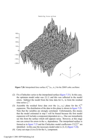


![Direct parameter estimation for SDOF systems 315
F
y y
´¾µ ´Ù½ Ù¾ µ for the 2DOF cubic oscillator.
Figure 7.23. Interpolated force surface ½
and the interpolated surface will contain spurious peaks.
These examples show that the Masri–Caughey method is a potentially
powerful means of identifying nearly arbitrary nonlinear systems. In their later
work, Masri and Caughey adopted a scheme which made use of direct least-
squares estimation to obtain the linear system matrices, while retaining the
Chebyshev expansion approach for the nonlinear forces [176, 177]. The following
sections discuss an approach based completely on direct least-squares methods
which shows some advantages over the hybrid approach.
7.4 Direct parameter estimation for SDOF systems
7.4.1 Basic theory
Certain disadvantages of the Masri–Caughey procedure may already have become
apparent: (i) it is time-consuming; (ii) there are many routes by which errors
Copyright © 2001 IOP Publishing Ltd](https://image.slidesharecdn.com/72268096-non-linearity-in-structural-dynamics-detection-identification-and-modelling-copy-120717010202-phpapp02/85/72268096-non-linearity-in-structural-dynamics-detection-identification-and-modelling-copy-331-320.jpg)


![318 System identification—continuous time
Figure 7.26. Comparison of measured data and that predicted by the Chebyshev model for
´½µ ´½µ
the 2DOF cubic oscillator: linear model with ½ and ¾ used.
If necessary, one can include in the model, basis functions for well-known
nonlinearities, i.e. × Ò´Ý µ for friction. This was first observed in [9].
As an aside, note that there is no reason why a model of the form
Ñ Ò
ÑÝ · Ì ´ÝµÌ ´Ýµ ܴص (7.60)
¼ ¼
should not be adopted, where Ì is the Chebyshev polynomial of order .
This means that DPE allows the determination of a Masri–Caughey-type model
without having to obtain the coefficients from double integrals. In fact, the
Chebyshev expansions are obtained much more quickly and with greater accuracy
by this method.
To simplify matters, the MSE used for direct least-squares is based on the
Copyright © 2001 IOP Publishing Ltd](https://image.slidesharecdn.com/72268096-non-linearity-in-structural-dynamics-detection-identification-and-modelling-copy-120717010202-phpapp02/85/72268096-non-linearity-in-structural-dynamics-detection-identification-and-modelling-copy-334-320.jpg)


![Direct parameter estimation for SDOF systems 321
(1)
h1
u1 u1
´½µ ´Ù½ Ù½ µ
Figure 7.29. Interpolated force surface ½ for the 3DOF piecewise linear
oscillator.
then identification (i.e. curve-fitting to) of the stiffness and damping sections is
sufficient to identify the whole system. Figures 7.37–7.39 show, respectively, the
sections for data from a linear system, a Duffing oscillator and a piecewise linear
system.
7.4.2.2 Crawley/O’Donnell surfaces
This method of constructing the force surfaces was introduced in [70, 71]. One
begins with the triplets obtained from the sampling and processing ´Ý Ý µ.
One then divides the rectangle in the phase plane Ý Ñ Ò ÝÑ Ü ¢ ÝÑ Ò ÝÑ Ü into
small grid squares. If a grid square contains sample points ´Ý Ý µ, the force
values above these points are averaged to give an overall force value for the
square. This gives a scattering of force values on a regular grid comprising the
Copyright © 2001 IOP Publishing Ltd](https://image.slidesharecdn.com/72268096-non-linearity-in-structural-dynamics-detection-identification-and-modelling-copy-120717010202-phpapp02/85/72268096-non-linearity-in-structural-dynamics-detection-identification-and-modelling-copy-337-320.jpg)


![Direct parameter estimation for SDOF systems 325
(2)
h1
u3 u1
Figure 7.33. Chebyshev model fit of order ´ µ to the surface in figure 7.32.
7.4.4 Identification of an impacting beam
The system of interest here is a beam made of mild steel, mounted vertically with
one encastr´ end and one free end as shown in figure 4.33. If the amplitude
e
of transverse motion of the beam exceeds a fixed limit, projections fixed on
either side of the beam make contact with a steel bush fixed in a steel cylinder
surrounding the lower portion of the beam. In the experiments described here, the
clearance was set at 0.5 mm. Clearly, when the beam is in contact with the bush,
the effective length of the beam is lowered with a consequent rise in stiffness.
Overall, for transverse vibrations, the beam has a piecewise linear stiffness. Initial
tests showed that the inherent damping of the beam was very light, so this was
augmented by the addition of constrained layer damping material to both sides of
the beam. Separate tests were carried out at low and high excitation.
7.4.4.1 Low excitation tests
The purpose of this experiment was to study the behaviour of the beam without
impacts, when it should behave as a linear system. Because of the linearity, the
experiment can be compared with theory. The dimensions and material constants
for the beam are given in table 7.4.
According to [42], the first two natural frequencies of a cantilever (fixed-
Copyright © 2001 IOP Publishing Ltd](https://image.slidesharecdn.com/72268096-non-linearity-in-structural-dynamics-detection-identification-and-modelling-copy-120717010202-phpapp02/85/72268096-non-linearity-in-structural-dynamics-detection-identification-and-modelling-copy-341-320.jpg)


![328 System identification—continuous time
y
y δy
fs (y)
y
f (y, 1 2 δ)
f (y, 1
2 δ)
Figure 7.36. Schematic diagram showing the formation of the stiffness section.
where the displacement Ý is obtained m from the free end. The mass Ñ´ µ is
fixed by the requirement that the natural frequency of the system is given by
½
´ µ ¾
Ò½ ¾ ½ (7.70)
Ñ´ µ
Two low level tests were carried out with the accelerometer at the direct-point
and cross-point. The instrumentation is shown in figure 7.47. Unfortunately, the
CED 1401 sampling instrument was not capable of sampling input and output
simultaneously, so the acceleration samples lagged the forces by ¡Ø ¾ with ¡Ø
the sampling interval. In order to render the two channels simultaneous, the
accelerations were shifted using an interpolation scheme [272].
The first test was carried out with the accelerometer at the cross-point; 5000
points were sampled at 500 Hz. The excitation was white noise band-limited into
the interval [10–20] Hz. The accelerations were integrated using the trapezium
rule to give velocities and displacements and the estimated signals were band-pass
filtered to eliminate spurious components from the integration (the procedures for
integration are discussed in some detail in appendix I).
Copyright © 2001 IOP Publishing Ltd](https://image.slidesharecdn.com/72268096-non-linearity-in-structural-dynamics-detection-identification-and-modelling-copy-120717010202-phpapp02/85/72268096-non-linearity-in-structural-dynamics-detection-identification-and-modelling-copy-344-320.jpg)


![Direct parameter estimation for SDOF systems 333
Figure 7.41. Crawley–O’Donnell surface for a linear system.
7.4.4.2 High excitation test
This test was carried out at the cross-point. The level of excitation was increased
until the projections on the side of the beam made contact with the bush. As
before, the input was band-limited into the range [10–20] Hz. The output
spectrum from the test showed a significant component at high frequencies, so
the sampling frequency for the test was raised to 2.5 kHz. The high-frequency
component made accurate time-shifting difficult, so it was not carried out; the
analysis in [272] indicates, in any case, that the main effect would be on the
damping, and the stiffness is of interest here. The data were integrated using the
trapezium rule and then filtered into the interval ½¼ ¾¼¼ in order to include a
sufficient number of harmonics in the data. A linear LS fit gave a mass estimate
of 2.24 kg which was used to form the restoring force. The stiffness section is
given in figure 7.49 (the force surface and damping section are not given as the
Copyright © 2001 IOP Publishing Ltd](https://image.slidesharecdn.com/72268096-non-linearity-in-structural-dynamics-detection-identification-and-modelling-copy-120717010202-phpapp02/85/72268096-non-linearity-in-structural-dynamics-detection-identification-and-modelling-copy-349-320.jpg)
![334 System identification—continuous time
Figure 7.42. Crawley–O’Donnell surface for a cubic stiffness system.
damping behaviour is biased). The section clearly shows the piecewise linear
behaviour with discontinuities at ¦¼ mm. This is acceptably close to the design
clearances of ¦¼ mm.
7.4.5 Application to measured shock absorber data
The automotive shock absorber or damper merits careful study as a fundamental
part of the automobile suspension system since the characteristics of the
suspension are a major factor in determining the handling properties and ride
comfort characteristics of a vehicle.
In vehicle simulations the shock absorber subsystem is usually modelled
as a simple linear spring-damper unit. However, experimental work by Lang
[157, 223], Hagedorn and Wallaschek [127, 262] and Genta and Campanile [108]
on the dynamics of shock absorbers in isolation show that the assumption of
Copyright © 2001 IOP Publishing Ltd](https://image.slidesharecdn.com/72268096-non-linearity-in-structural-dynamics-detection-identification-and-modelling-copy-120717010202-phpapp02/85/72268096-non-linearity-in-structural-dynamics-detection-identification-and-modelling-copy-350-320.jpg)
![Direct parameter estimation for SDOF systems 335
Figure 7.43. Crawley–O’Donnell surface for a piecewise linear system.
linearity is unjustified. This is not a surprising conclusion as automotive dampers
are designed to have different properties in compression and rebound in order to
give balance to the handling and comfort requirements.
On recognizing that the absorber is significantly nonlinear, some means of
characterizing this nonlinearity is needed, in order that the behaviour can be
correctly represented in simulations.
The most careful theoretical study of an absorber is that of Lang [157]. A
physical model was constructed which took properly into account the internal
compressive oil/gas flow through the various internal chambers of the absorber;
the result was an 87 parameter, highly nonlinear model which was then simulated
using an analogue computer; the results showed good agreement with experiment.
Unfortunately Lang’s model necessarily depends on the detailed construction of
a particular absorber and cannot be applied to any other.
Rather than considering the detailed physics, a more straightforward
Copyright © 2001 IOP Publishing Ltd](https://image.slidesharecdn.com/72268096-non-linearity-in-structural-dynamics-detection-identification-and-modelling-copy-120717010202-phpapp02/85/72268096-non-linearity-in-structural-dynamics-detection-identification-and-modelling-copy-351-320.jpg)

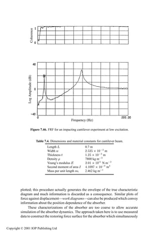

![Direct parameter estimation for SDOF systems 339
Figure 7.48. Estimated restoring force surface for the impacting cantilever at a low level
of excitation.
model of the structure. If necessary, a parametric model can be fitted using the LS
methods described earlier or the Masri–Caughey procedure.
The restoring force surface procedure has been applied to the identification
of automotive shock absorbers in a number of publications [16, 19, 239]. The
most recent work [82] is noteworthy as it also generated fundamental work on
restoring force surfaces in general, firstly a new local definition of the surface has
been proposed, which fits different models over different sections of the phase
plane [83]. Secondly, it has been possible to generate optimal input forces for
restoring force surface identification [84].
The results presented here are for a number of sets of test data from a
FIAT vehicle shock absorber. The data were obtained by FIAT engineers using
the experimental facilities of the vehicle test group at Centro Ricerche FIAT,
Orbassano. The apparatus and experimental strategy are shown in figure 7.51 and
are described in more detail in [19]; the subsequent data processing and analysis
can be found in [239]. Briefly, data were recorded from an absorber which was
constrained to move in only one direction in order to justify the assumption of
SDOF behaviour. The top of the absorber was fixed to a load cell so that the
internal force could be measured directly (it was found that inertial forces were
Copyright © 2001 IOP Publishing Ltd](https://image.slidesharecdn.com/72268096-non-linearity-in-structural-dynamics-detection-identification-and-modelling-copy-120717010202-phpapp02/85/72268096-non-linearity-in-structural-dynamics-detection-identification-and-modelling-copy-355-320.jpg)
![340 System identification—continuous time
Figure 7.49. Estimated stiffness section for the impacting cantilever at a high level of
excitation.
negligible). The base was then excited harmonically using a hydraulic actuator.
The absorber was tested at six frequencies, 1, 5, 10, 15, 20, and 30 Hz; the results
shown here are for the 10 Hz test showing a range of amplitude levels.
The restoring force surface and the associated contour map are given in
figure 7.52, they both show a very clear bilinear characteristic. On the contour
map, the contours, which are concentrated in the positive velocity half-plane, are
parallel to each other and to the Ý ¼ axis showing that the position dependence
of the absorber is small. Note that if a parametric representation of the internal
force had been obtained, say a LS polynomial, it would have been impossible
to infer the bilinear characteristic from the coefficients alone; it is the direct
visualization of the nonlinearity which makes the force surface so useful.
The surfaces from the tests at other frequencies showed qualitatively the
same characteristics, i.e. a small linear stiffness and a bilinear damping. However,
the line of discontinuity in the surface was found to rotate in the phase plane as
the test frequency increased. A simple analysis using differenced force surfaces
showed that this dependence on frequency was not simply a consequence of
disregarding the absorber mass [274]. Force surfaces have also been used to
investigate the temperature dependence of shock absorbers [240].
Copyright © 2001 IOP Publishing Ltd](https://image.slidesharecdn.com/72268096-non-linearity-in-structural-dynamics-detection-identification-and-modelling-copy-120717010202-phpapp02/85/72268096-non-linearity-in-structural-dynamics-detection-identification-and-modelling-copy-356-320.jpg)


![Direct parameter estimation for MDOF systems 345
In principle, the inclusion of difference variables allows the model to locate
nonlinearity [9]; for example, if a term of the form ´Æ ¾¿ µ¿ appears in the
appropriate expansion one can infer the presence of a cubic stiffness nonlinearity
between points 2 and 3.
Suppose now that only one of the inputs Ü is non-zero. Without loss of
generality it can be taken as Ü ½ . The equations of motion become
Æ
ѽ Ý · ´Æ Æ µ ܽ ´Øµ (7.78)
½
Æ
Ý · ¼ ´Æ Æ µ ¼ ¾ Æ (7.79)
½
One can identify all coefficients in the Ý ¾ equation up to an overall scale—the
¼
unknown Ñ ¾ which is embedded in each ¾ . Similarly, all the coefficients in the
Ý¿ equation can be known up to the scale Ñ ¿ . Multiplying the latter coefficients
by the ratio Ѿ Ñ¿ would therefore scale them with respect to Ñ ¾ . This means
that coefficients for both equations are known up to the same scale Ñ ¾ . The ratio
Ѿ Ñ¿ can be obtained straightforwardly; if there is a link Ð ¾¿ the two equations
¼ ¼
will contain terms ¾¿ and ¿¾ . Choosing one particular term, e.g. the linear
stiffness term, from each ¼ expansion gives, via (7.77)
Ѿ ¼
´¿¾µ½¼
Ñ¿ ¼ (7.80)
´¾¿µ¼½
The scale Ѿ can then be transferred to the Ý equation coefficients by the
same method if there is a link Ð ¾ or п . In fact, the scale factor can be propagated
through all the equations since each mass point must be connected to all other
mass points through some sequence of links. If this were not true the system
would fall into two or more disjoint pieces.
If the ݽ equation has an input, Ñ ½ is estimated and this scale can be
transferred to all equations so that the whole MDOF system can be identified
using only one input. It was observed in [283] that if the unforced equations of
motion are considered, the required overall scale can be fixed by a knowledge
of the total system mass, i.e. all system parameters can be obtained from
measurements of the free oscillations.
If a restriction is made to linear systems, the equations and notation can be
simplified a great deal. Substituting
´ µ¼½ (7.81)
´ µ½¼ (7.82)
in the linear versions of the equations of motion (7.78) and (7.79) yields
Æ Æ
ѽ Ý · Æ · Æ Ü½ ´Øµ (7.83)
½ ½
Copyright © 2001 IOP Publishing Ltd](https://image.slidesharecdn.com/72268096-non-linearity-in-structural-dynamics-detection-identification-and-modelling-copy-120717010202-phpapp02/85/72268096-non-linearity-in-structural-dynamics-detection-identification-and-modelling-copy-361-320.jpg)
![346 System identification—continuous time
Æ Æ
Ý · ¼ Æ · ¼Æ ¼ ¾ Æ (7.84)
½ ½
where ¼ Ñ and ¼ Ñ.
If estimates for Ñ , and are obtained, then the usual stiffness and
damping matrices and are recovered from the simple relations
Æ Æ
(7.85)
½ ½
The symmetry conditions (7.76) become
(7.86)
which imply
(7.87)
so the model structure forces a symmetry or reciprocity condition on the damping
and stiffness matrices. By assuming that reciprocity holds at the outset, it is
possible to identify all system parameters using one input by an alternative
method which is described in [189].
A further advantage of adopting this model is that it allows a natural
definition of the restoring force surface for each link. After obtaining the model
coefficients the surface can be plotted as a function of Æ and Æ for each link
Ð . In this case the surfaces are purely a visual aid to the identification, and are
more appropriate in the nonlinear case.
7.5.2 Experiment: linear system
The system used for the experiment was a mild steel cantilever (fixed-free) beam
mounted so that its motion was confined to the horizontal plane. In order to
make the system behave as far as possible like a 3DOF system, three lumped
masses of 0.455 kg each, in the form of mild steel cylinders, were attached to
the beam at equally spaced points along its length (figure 7.54). The system
was described in [111] where a functional-series approach was used in order
to identify the characteristics of such systems as discussed in the next chapter.
Initial tests showed the damping in the system to be very low; to increase the
energy dissipation, constrained layer damping material was fixed to both sides of
the beam in between the cylinders.
Details of the various geometrical and material constants for the system
are given in [189] in which an alternative approach to DPE is used to analyse
data from this system. In order to obtain theoretical estimates of the natural
frequencies etc, estimates of the mass matrix Ñ and the stiffness matrix are
Copyright © 2001 IOP Publishing Ltd](https://image.slidesharecdn.com/72268096-non-linearity-in-structural-dynamics-detection-identification-and-modelling-copy-120717010202-phpapp02/85/72268096-non-linearity-in-structural-dynamics-detection-identification-and-modelling-copy-362-320.jpg)
![Direct parameter estimation for MDOF systems 347
CED 1401
x y3
y1 y2
v1 v2 v3 v4
Charge
Amplifiers
Accelerometers
m1 m2 m3
Force Transducer
Shaker
Amplifier
Filter
Signal
Generator
Figure 7.54. Instrumentation for the restoring force surface experiments on the 3DOF
experimental nonlinear system.
needed. Assuming that the system can be treated as a 3DOF lumped parameter
system, the mass is assumed to be concentrated at the locations of the cylinders.
The mass of the portion of beam nearest to each cylinder is transferred to the
cylinder. The resulting estimate of the mass matrix was
Ñ ¼ ¼ ¼¼¼¼ ¼ ¼¼¼¼ [kg]
¼ ¼¼¼¼ ¼ ¼ ¼¼¼¼
¼ ¼¼¼¼ ¼ ¼¼¼¼ ¼ ½
Simple beam theory yielded an estimate of the stiffness matrix
½¼ ¢ ½¾ ¼ ¾¿¿ ¼½ N m ½
¼ ¾¿¿ ¼ ½ ¼ ¾ ½
¼½ ¼ ¾ ½ ¼ ½½¼½
Copyright © 2001 IOP Publishing Ltd](https://image.slidesharecdn.com/72268096-non-linearity-in-structural-dynamics-detection-identification-and-modelling-copy-120717010202-phpapp02/85/72268096-non-linearity-in-structural-dynamics-detection-identification-and-modelling-copy-363-320.jpg)
![348 System identification—continuous time
Having obtained these estimates, the eigenvalue problem
¾Ñ (7.88)
was solved, yielding the natural frequencies ¾ and the modeshapes
. The predictions for the first three natural frequencies were 4.76, 22.34,
and 77.11 Hz. As the integrating procedures used to obtain velocity and
displacement data from measured accelerations require a band-limited input to
be used, it would have proved difficult to excite the first mode and still have
no input at low frequencies. For this reason, a helical compression spring with
stiffness 1.106¢½¼ N m ½ was placed between point 3 and ground as shown
in figure 7.54. The added mass of the spring was assumed to be negligible.
The modification to the stiffness matrix was minimal, except that ¿¿ changed
from ½ ½¼½ ¢ ½¼ to ¾ ¾¼ ¢ ½¼ . However, the first natural frequency changed
dramatically, re-solving the eigenvalue problem gave frequencies of 17.2, 32.0
and 77.23 Hz.
The arrangement of the experiment is also shown in figure 7.54. The signals
were sampled and digitized using a CED 1401 intelligent interface. A detailed
description of the rest of the instrumentation can be found in [267].
The first experiment carried out on the system was a modal analysis
to determine accurately the natural frequencies of the system. The FRFs
½ ´ µ ´ µ, ¾ ´ µ ´ µ and ¿ ´ µ ´ µ were obtained; standard curve-
fitting to these functions showed that the first three natural frequencies were
16.91, 31.78 and 77.78 Hz in good agreement with the theoretical estimates. The
averaged output spectrum for the system when excited by a band-limited input
in the range 10–100 Hz is shown in figure 7.55; there seems to be no significant
contribution from higher modes than the third and it would therefore be expected
that the system could be modelled well by a 3DOF model if the input is band-
limited in this way.
An experiment was then carried out with the intention of fitting LS models of
the types (7.77) and (7.78) to the data. The excitation used was a noise sequence
band-limited in the range 10–100 Hz. The data ܴص, Ý ½ , ݾ and Ý¿ were sampled
with frequency 1666.6 Hz, and 3000 points per channel were taken. Equal-
interval sampling between channels was performed.
The acceleration signals were integrated using the trapezium rule followed
by band-pass filtering in the range 10–100 Hz [274]; the data were passed through
the filter in both directions in order to eliminate phase errors introduced by a
single pass. To remove any filter transients 500 points of data were deleted from
the beginning and end of each channel; this left 2000 points per channel.
An inhomogeneous ´½ ½µ model was fitted to data points 500 to 1500 in
order to identify the Ý ½ equation of motion; the result was
¼ ݽ ¿¿Ý½ · ¢ ½¼ ݽ · ½¼ ½´Ý½ ݾ µ
· ¿¿ ¢ ½¼ ´Ý½ ݾ µ ¾ ¾¿ ¢ ½¼ ´Ý½ Ý¿ µ ܴص (7.89)
Copyright © 2001 IOP Publishing Ltd](https://image.slidesharecdn.com/72268096-non-linearity-in-structural-dynamics-detection-identification-and-modelling-copy-120717010202-phpapp02/85/72268096-non-linearity-in-structural-dynamics-detection-identification-and-modelling-copy-364-320.jpg)
![Direct parameter estimation for MDOF systems 349
Figure 7.55. Output spectrum for the linear 3DOF system under excitation by a random
signal in the range 10–100 Hz.
Comparing the predicted and measured data gave an MSE of 0.035%, indicating
excellent agreement. In all models for this system the significance threshold for
deleting insignificant terms was set at 0.1%.
A homogeneous ´½ ½µ model was fitted to each of the Ý ¾ and Ý¿ equations
of motion. The results were
ݾ · ½½ ¢ ½¼ ´Ý¾ ݽ µ ¿ ¢ ½¼ ݾ · ¿ ¿ ¢ ½¼ ´Ý¾ Ý¿ µ ¼ (7.90)
and
Ý¿ · ´Ý¿ ݽ µ ½¿Ý¿ ¿ ¢ ½¼ ´Ý¿ ݽ µ
· ¿ ¢ ½¼ ´Ý¿ ݾ µ · ¿ ¼¼ ¢ ½¼ Ý¿ ¼ (7.91)
The comparisons between measured and predicted data gave MSE values of
0.176% and 0.066%, again excellent.
The scale factors were transferred from the first equation of motion to the
others as previously described. The final results for the (symmetrized) estimated
system matrices were
Ñ ¼ ¼ ¼¼¼¼ ¼ ¼¼¼¼ [kg]
¼ ¼¼¼¼ ¼ ½ ¾ ¼ ¼¼¼¼
¼ ¼¼¼¼ ¼ ¼¼¼¼ ¼ ¼¼
Copyright © 2001 IOP Publishing Ltd](https://image.slidesharecdn.com/72268096-non-linearity-in-structural-dynamics-detection-identification-and-modelling-copy-120717010202-phpapp02/85/72268096-non-linearity-in-structural-dynamics-detection-identification-and-modelling-copy-365-320.jpg)
![350 System identification—continuous time
Table 7.5. Natural frequencies for linear system.
Experimental Model
frequency frequency Error
Mode (Hz) (Hz) (%)
1 16.914 17.044 0.77
2 31.781 32.247 1.47
3 77.529 77.614 0.11
½¼ ¢ ½¿ ¼ ¿¿ ¼ ¾¾¿¿ N m ½
¼ ¿¿ ¼ ¼ ¾
¼ ¾¾¿¿ ¼ ¾ ¼ ¾¿
which compare favourably with the theoretical results. In all cases, the damping
estimates have low significance factors and large standard deviations, indicating
a low level of confidence. This problem is due to the low level of damping in
the system, the constrained layer material having little effect. Thus the damping
matrix estimates are not given. Using the estimated Ñ and matrices, the first
three natural frequencies were estimated. The results are shown in table 7.5 and
the agreement with the modal test is good. However, the question remains as to
whether the parameters correspond to actual physical masses and stiffnesses. In
order to address this question, another experiment was carried out. An additional
1 kg mass was attached to measurement point 2 and the previous experimental
procedure was repeated exactly. The resulting parameter estimates were
Ñ ¼ ¼ ¼¼¼¼ ¼ ¼¼¼¼ [kg]
¼ ¼¼¼¼ ½ ¾ ¼ ¼¼¼¼
¼ ¼¼¼¼ ¼ ¼¼¼¼ ¼ ¼
½¼ ¢ ½ ¿ ¼ ¼ ¼ ¼ ¾¾ N m ½
¼ ¼ ¼ ½ ¼ ¿¼½
¼ ¾¾ ¼ ¿¼½ ¼ ¾
and the results have changed very little from the previous experiment, the only
exception being that Ñ ¾¾ has increased by 1.01 kg. The results give confidence
that the parameters are physical for this highly discretized system with very small
effects from out-of-range modes. The natural frequencies were estimated and
compared with those obtained by curve-fitting to transfer functions. The results
are shown in table 7.6, again with good agreement.
7.5.3 Experiment: nonlinear system
The final experimental system was based on that in [111]. The same
experimental arrangement as in the previous subsection was used with a number
Copyright © 2001 IOP Publishing Ltd](https://image.slidesharecdn.com/72268096-non-linearity-in-structural-dynamics-detection-identification-and-modelling-copy-120717010202-phpapp02/85/72268096-non-linearity-in-structural-dynamics-detection-identification-and-modelling-copy-366-320.jpg)


![Direct parameter estimation for MDOF systems 353
Figure 7.57. Comparison of measured data and that predicted by the nonlinear model for
the second equation of motion for the nonlinear 3DOF experimental system.
A comparison between measured and predicted output gave an MSE of
0.31%, indicating that a linear model is adequate. To check, a ´¿ ¿µ model was
fitted and all but the linear terms were discarded as insignificant.
After transferring scales from the Ý ½ equation to the other two, the system
matrices could be constructed from the previous estimates. The symmetricized
results were
Ñ ¼ ¾¼ ¼ ¼¼¼¼ ¼ ¼¼¼¼ [kg]
¼ ¼¼¼¼ ¼ ¼ ¼¼¼¼
¼ ¼¼¼¼ ¼ ¼¼¼¼ ¼ ¼
½¼ ¢ ½ ¾ ¼ ¼ ¼ ¼ ¾¿½¼ N m ½
¼ ¼ ¼ ¼ ¼ ¾ ½½
¼ ¾¿½¼ ¼ ¾ ½½ ¼ ¾¿
These parameters show good agreement with those for the linear experiment. This
time, a significant damping coefficient ¾¾ was obtained; this is due to the linear
damping introduced by the shaker.
All that remained to be done now was to determine the true cubic coefficient
Copyright © 2001 IOP Publishing Ltd](https://image.slidesharecdn.com/72268096-non-linearity-in-structural-dynamics-detection-identification-and-modelling-copy-120717010202-phpapp02/85/72268096-non-linearity-in-structural-dynamics-detection-identification-and-modelling-copy-369-320.jpg)
![354 System identification—continuous time
Figure 7.58. Restoring force surface for link о½ in the nonlinear 3DOF experimental
system.
in the experiment. The details of this calibration experiment are given in [267].
The result was
¿¾¾¼ ¼Ý¾ ¿ (7.95)
The coefficient value estimated by the identification procedure was ¿½ ¦
½¼. The percentage error is therefore 69%; while this is a little high, the
estimate has the right order of magnitude and the error interval of the estimate
encloses the ‘true’ value.
The DPE scheme has also been implemented for distributed systems in [165].
It is clear that restoring force methods allow the identification of MDOF
nonlinear experimental systems. It should be stressed that high-quality instru-
mentation for data acquisition is required. In particular, poor phase-matching
between sampled data channels can result in inaccurate modelling of damping
behaviour. The two approaches presented here can be thought of as complemen-
tary. The Masri–Caughey modal coordinate approach allows the construction of
restoring force surfaces without specifying an a priori model. The main disadvan-
tage is that the surfaces are distorted by nonlinear interference terms from other
coordinates unless modes are well separated. The DPE approach produces force
Copyright © 2001 IOP Publishing Ltd](https://image.slidesharecdn.com/72268096-non-linearity-in-structural-dynamics-detection-identification-and-modelling-copy-120717010202-phpapp02/85/72268096-non-linearity-in-structural-dynamics-detection-identification-and-modelling-copy-370-320.jpg)
![System identification using optimization 355
Figure 7.59. Restoring force surface for link о¾ in the nonlinear 3DOF experimental
system.
surfaces only after a parametric model has been specified and fitted, but offers the
advantage that systems with close modes present no particular difficulties.
7.6 System identification using optimization
The system identification methods discussed earlier in this chapter and the
previous one are only appropriate for linear-in-the-parameters system models
and, although these form a large class of models, they by no means exhaust the
possibilities. Problems begin to arise when the system nonlinearity is not linear-
in-the-parameters, e.g. for piecewise-linear systems (which include clearance,
deadband and backlash systems) or if the equations of motion contain states which
cannot be measured directly, e.g. in the Bouc–Wen hysteresis model discussed
later. If the objective function for optimization, e.g. squared-error, depends
differentiably on the parameters, traditional minimization techniques like gradient
descent or Gauss–Newton [99] can be used. If not, newly developed (or rather,
newly exploited) techniques like genetic algorithms (GAs) [117] or downhill
simplex [209] can be employed. In [241], a GA with simulated annealing was
used to identify linear discrete-time systems. In [100], the GA was used to find the
Copyright © 2001 IOP Publishing Ltd](https://image.slidesharecdn.com/72268096-non-linearity-in-structural-dynamics-detection-identification-and-modelling-copy-120717010202-phpapp02/85/72268096-non-linearity-in-structural-dynamics-detection-identification-and-modelling-copy-371-320.jpg)
![356 System identification—continuous time
Figure 7.60. Restoring force surface for link о¿ in the nonlinear 3DOF experimental
system.
structure for an NARMAX model. This section demonstrates how optimization
methods, GAs and gradient descent, in particular, can be used to solve continuous-
time parameter estimation problems.
7.6.1 Application of genetic algorithms to piecewise linear and hysteretic
system identification
7.6.1.1 Genetic algorithms
For the sake of completeness, a brief discussion of genetic algorithms (GAs) will
be given here, for more detail the reader is referred to the standard introduction to
the subject [117].
GAs are optimization algorithms developed by Holland [132], which evolve
solutions in a manner based on the Darwinian principle of natural selection. They
differ from more conventional optimization techniques in that they work on whole
populations of encoded solutions. Each possible solution, in this case each set of
possible model parameters, is encoded as a gene. The most usual form for this
gene is a binary string, e.g. 0001101010 gives a 10-bit (i.e. accurate to one part
in 1024) representation of a parameter. In this illustration, two codes were used:
Copyright © 2001 IOP Publishing Ltd](https://image.slidesharecdn.com/72268096-non-linearity-in-structural-dynamics-detection-identification-and-modelling-copy-120717010202-phpapp02/85/72268096-non-linearity-in-structural-dynamics-detection-identification-and-modelling-copy-372-320.jpg)
![System identification using optimization 357
the first which will be called the interval code, is obtained by multiplying a small
number ¡Ô by the integer obtained from the bit-string, for each parameter Ô .
The second code, the range code, is obtained by mapping the expected range of
the parameter onto [¼ ½¼¾¿] for example.
Having decided on a representation, the next step is to generate, at random,
an initial population of possible solutions. The number of genes in a population
depends on several factors, including the size of each individual gene, which itself
depends on the size of the solution space.
Having generated a population of random genes, it is necessary to decide
which of them are fittest in the sense of producing the best solutions to the
problem. To do this, a fitness function is required which operates on the encoded
genes and returns a single number which provides a measure of the suitability
of the solution. These fitter genes will be used for mating to create the next
generation of genes which will hopefully provide better solutions to the problem.
Genes are picked for mating based on their fitnesses. The probability of a
particular gene being chosen is equal to its fitness divided by the sum of the
fitnesses of all the genes in the population. Once sufficient genes have been
selected for mating, they are paired up at random and their genes combined to
produce two new genes. The most common method of combination used is called
crossover. Here, a position along the genes is chosen at random and the substrings
from each gene after the chosen point are switched. This is one-point crossover. In
two-point crossover a second position is chosen and the gene substrings switched
again. There is a natural fitness measure for identification problem, namely the
inverse of the comparison error between the reference data and the model data
(see later).
The basic problem addressed here is to construct a mathematical model of
an input–output system given a sampled-data record of the input time series ܴص
and the corresponding output series Ý ´Øµ (for displacement say). The ‘optimum’
model is obtained by minimizing the error between the reference data Ý ´Øµ, and
that produced by the model Ý ´Øµ when presented with the sequence ܴص. The
error function used here is the MSE defined in (6.108), the fitness for the GA is
obtained simply by inverting the MSE.
If a gene in a particular generation is extremely fit, i.e. is very close to the
required solution, it is almost certain to be selected several times for mating. Each
of these matings, however, involves combining the gene with a less fit gene so the
maximum fitness of the population may be lower in the next generation. To avoid
this, a number of the most fit genes can be carried through unchanged to the next
generation. These very fit genes are called the elite.
To prevent a population from stagnating, it can be useful to introduce
perturbations into the population. New entirely random genes may be added at
each generation. Such genes are referred to as new blood. Also, by analogy with
the biological process of the same name, genes may be mutated by randomly
switching one of their binary digits with a small probability. The mutation used
here considers each bit of each gene separately for switching.
Copyright © 2001 IOP Publishing Ltd](https://image.slidesharecdn.com/72268096-non-linearity-in-structural-dynamics-detection-identification-and-modelling-copy-120717010202-phpapp02/85/72268096-non-linearity-in-structural-dynamics-detection-identification-and-modelling-copy-373-320.jpg)
![358 System identification—continuous time
400.0
Excitation x(t) [N]
200.0
0.0
-200.0
-400.0
0.0 2000.0 4000.0 6000.0 8000.0 10000.0
Time (Sampling Instants)
0.004
Displacement y(t) [m]
0.002
0.000
-0.002
-0.004
-0.006
0.0 200.0 400.0 600.0 800.0 1000.0
Time (Sampling Instants / 10 )
Figure 7.61. Force and displacement reference data for genetic algorithm (GA)
identification of a linear system.
With genetic methods it is not always possible to say what the fitness of
a perfect gene will be. Thus the iterative process is usually continued until the
population is dominated by a few relatively fit genes. One or more of these genes
will generally be acceptable as solutions.
7.6.1.2 A linear system
Before proceeding to nonlinear systems, it is important to establish a benchmark,
so the algorithm is applied to data from a linear system. For simplicity, the
systems considered here are all single-degree-of-freedom (SDOF); this does not
represent a limitation of the method. Input and output data were obtained for the
system given by
ÑÝ · Ý · Ý Ü´Øµ (7.96)
with Ñ ½ kg, ¾¼ N s m ½ and ½¼ N m ½ , using a fourth-order
Runge–Kutta routine. ܴص was a sequence of 10 000 points of Gaussian white
noise with rms 75.0 and time step 0.0002. The resulting Ý ´Øµ was decimated by a
factor of 10 giving 1000 points of reference data with sampling frequency 500 Hz.
The data are shown in figure 7.61.
The methods of identifying this system shown previously in this chapter
would require the availability of displacement, velocity and acceleration data. An
advantage of the current method is the need for only one response variable.
Copyright © 2001 IOP Publishing Ltd](https://image.slidesharecdn.com/72268096-non-linearity-in-structural-dynamics-detection-identification-and-modelling-copy-120717010202-phpapp02/85/72268096-non-linearity-in-structural-dynamics-detection-identification-and-modelling-copy-374-320.jpg)


![System identification using optimization 361
f(y)
k2
y
d
k1
Figure 7.65. Simulated bilinear stiffness under investigation using the GA.
7.6.1.3 A piecewise linear system
The first nonlinear system considered here is a bilinear system with equation of
motion
ÑÝ · Ý · ´Ýµ ܴص (7.97)
with Ñ and as before. ´Ýµ has the form (figure 7.65)
´Ý µ ½Ý Ý
½ · ¾ ´Ý µ
(7.98)
Ý
with ½ ½¼¼¼ ¼, ¾ ½¼ ¼¼¼ ¼ and ¼ ¼¼½. This system is only
physically sensible, i.e. ´Ý µ goes through the origin, if is positive. This
is not a restriction, in the general case, one could allow several negative and
positive break points. It is the complicated dependence on which makes ´Ý µ a
problem for standard parameter estimation routines. However, there is essentially
nothing to distinguish this system from the linear one from the point of view
of the GA. The only difference is that five parameters are needed, so a 50-bit
gene is required if the same precision is retained. In this experiment, the same
GA parameters as before were used but the code was the range code and linear
fitness scaling was used [117]. The ranges were ¼ ½¼¼ for Ñ and , ¼ ¾¼ ¼¼¼
for ½ and ¾ and ¼ ¼¾ ¼ ¼¾ for . Displacement was used for this run as
the bilinear stiffness produces a significant mean level in the displacement which
might provide a useful feature for the identification. The GA obtained a solution
after 250 generations with Ñ ¼ ¾, ½ ½, ½ ¿ ½, ¾ ½¼ ¼¾
and ¼ ¼¼½ ¼ and then failed to refine this further. The resulting comparison
of model and reference data gave an MSE of 0.19.
To improve the solution, the GA was run again with the ranges taken from
the final population of the previous run. The ranges were ¼ ¾ ½ ½ for
Ñ, ½ ½ ¾½ for , ¿¼ ¿ ½½ for ½ , ¿ ½½ ¾ ½ for ¾ and
¼ ¼¼¼ ¼ ¼½¿ for . All other GA parameters were retained. The GA
attained a fitness of 205.8 after 400 generations, corresponding to an MSE of
Copyright © 2001 IOP Publishing Ltd](https://image.slidesharecdn.com/72268096-non-linearity-in-structural-dynamics-detection-identification-and-modelling-copy-120717010202-phpapp02/85/72268096-non-linearity-in-structural-dynamics-detection-identification-and-modelling-copy-377-320.jpg)
![362 System identification—continuous time
0.010
Reference Data
Fittest Gene
Displacement y(t) [m]
0.000
-0.010
-0.020
0.0 200.0 400.0 600.0 800.0 1000.0
Time (Sampling Instants / 10)
Figure 7.66. Comparison of measured and predicted displacements from GA identification
of the bilinear system.
0.005. The final parameters were Ñ ½ ¼½ , ¾¼ ¼¿, ½ ½¼¼ ¼,
¾ ½¼ ¿¼¼ ¼ and ¼ ¼¼½. A comparison between model and reference
data is given in figure 7.66, the two traces are indistinguishable.
7.6.1.4 A hysteretic system
The Bouc–Wen model [44, 263], briefly discussed before, is a general nonlinear
hysteretic restoring force model where the total restoring force É´Ý Ý µ is
composed of a polynomial non-hysteretic and a hysteretic component based on
the displacement time history. A general hysteretic system described by Wen is
represented next, where ´Ý ݵ is the polynomial part of the restoring force and
Þ ´Ýµ the hysteretic:
ܴص ÑÝ · Þ ´Ý ݵ (7.99)
É´Ý Ýµ ´Ý ݵ · Þ ´Ýµ (7.100)
´Ý ݵ ´Ýµ · ´Ýµ (7.101)
Where the polynomial function ´Ý ݵ is separated into its displacement and
velocity components
´Ýµ ¼ × Ò´Ýµ · ½ Ý · ¾ Ý Ý · ¿ Ý¿ · ¡ ¡ ¡ (7.102)
´Ý µ ¼ × Ò´Ýµ · ½ Ý · ¾ Ý Ý · ¿ Ý¿ · ¡ ¡ ¡ (7.103)
The system under test here is an SDOF system based on this model with
´Ý ݵ ¼ for simplicity as studied in [178] ܴص is a random force, with the
Copyright © 2001 IOP Publishing Ltd](https://image.slidesharecdn.com/72268096-non-linearity-in-structural-dynamics-detection-identification-and-modelling-copy-120717010202-phpapp02/85/72268096-non-linearity-in-structural-dynamics-detection-identification-and-modelling-copy-378-320.jpg)
![System identification using optimization 363
hysteretic component Þ ´Ý µ defined in [263] by
Þ « Ý Þ Ò ¬ Ý Þ Ò · Ý for Ò odd
« Ý Þ Ò ½ Þ ¬ ÝÞ Ò · Ý for Ò even.
(7.104)
This may be reduced to
Þ
Ü
¦ ´« ¦ ¬ µÞ Ò (7.105)
Equation (7.105) may be integrated in closed form to show the hysteretic
relationship between Þ and Ý where « ¬ and Ò are the constants that govern
the scale, shape and smoothness of the hysteresis loop.
A series of experiments were performed using the GA to identify the
parameters of a Bouc–Wen based SDOF system as presented earlier. The
parameters of the reference system were Ñ ½ ¼ kg, Ò ¾, « ½ N ½ Ò m ½ ,
¬ ½ N½ Ò m ½ and ¼ ¼ N m ½ . The reference system (figure 7.67)
and the systems generated from the GA runs were driven with the same Gaussian
noise input signal with an rms value of 10.0 N. Reference and experimental data
were compared on 2000 data points using the MSE of the displacement data.
The fitness score for each gene was obtained by the reciprocal of the MSE as
before. Genes whose parameters matched exactly those of the reference system
resulted in a ‘divide by zero’ which was one test condition for termination of the
program. Genes that described systems that produced outputs either falling to
zero or exploding to infinity were assigned a zero-fitness score.
The data were sampled at 250 Hz giving a step size of ¼ ¼¼ . The results
included in figures 7.68–7.70 are from the same GA test run with the following
parameters.
Population size 500
Gene length 62
Number of generation 100
Crossover type two-point
Crossover probability 80%
Mutation probability 10%
Number of elite genes 1
Number of new blood 50.
The peak fitness achieved by a gene in the test run was 4.53 giving a
corresponding MSE of ¼ ¾¾±. Figure 7.68 is given to compare the displacement
signals of the reference and test system, the plots overlay. Figure 7.69 shows a
comparison of the hysteresis loops.
The results shown are the best of many GA runs made while good simulation
parameters were being determined. The average GA run achieved a lower fitness
than this, but with results still being in the region of only 1% error.
The parameters decoded from the fittest gene in this case were as in table 7.7.
The peak fitness was achieved near the 35th generation of the test. Table 7.7
shows the final output from the run after 100 generations. Figure 7.70 shows the
Copyright © 2001 IOP Publishing Ltd](https://image.slidesharecdn.com/72268096-non-linearity-in-structural-dynamics-detection-identification-and-modelling-copy-120717010202-phpapp02/85/72268096-non-linearity-in-structural-dynamics-detection-identification-and-modelling-copy-379-320.jpg)
![364 System identification—continuous time
40.0
20.0
x(t) [N]
0.0
-20.0
-40.0
0.0 500.0 1000.0 1500.0 2000.0
Sampling Instants
(a)
0.010
0.005
Displacement y [m]
0.000
-0.005
-0.010
0.0 500.0 1000.0 1500.0 2000.0
Sampling Instants
(b)
Figure 7.67. Force and displacement reference data for GA identification of the hysteretic
system.
Copyright © 2001 IOP Publishing Ltd](https://image.slidesharecdn.com/72268096-non-linearity-in-structural-dynamics-detection-identification-and-modelling-copy-120717010202-phpapp02/85/72268096-non-linearity-in-structural-dynamics-detection-identification-and-modelling-copy-380-320.jpg)

![366 System identification—continuous time
10.0
1.0
Fitness
0.1
0.0
Maximum Fitness
Average Fitness
0.0
0.0 20.0 40.0 60.0 80.0 100.0
Generation Number
Figure 7.70. Evolution of fitness for GA identification of the linear system.
Table 7.7. Best parameter from GA for hysteretic system.
Parameter Reference Best gene Error (%)
Ñ 1.00 0.97 3
Ò 2 2 0
« 1.50 1.64 9
¬ 1.50 1.75 17
6680 6450 4
maximum; this is a result of the high mutation rates that were used to prevent
premature population stagnation.
The method is an improvement on that of [178], in which it was assumed that
Ñ was known. The advantage of this assumption is that it allows the separation of
the Þ -variable and reduces the problem to a linear-in-the-parameters estimation;
this, however, is unrealistic.
Optimization, and GAs in particular, provide an attractive means of
estimating parameters for otherwise troublesome systems. Physical parameters
are obtained without going through a discrete model or using costly
instrumentation or signal processing to generate displacement, velocity and
acceleration data. It is a simple matter to use the algorithm with any of these
Copyright © 2001 IOP Publishing Ltd](https://image.slidesharecdn.com/72268096-non-linearity-in-structural-dynamics-detection-identification-and-modelling-copy-120717010202-phpapp02/85/72268096-non-linearity-in-structural-dynamics-detection-identification-and-modelling-copy-382-320.jpg)
![System identification using optimization 367
response types. The GA is not unique in this respect, any optimization engine
could be used here which uses a single scalar objective function and does not
require gradients or Hessians. Downhill simplex or simulated annealing should
produce similar results. The method could be used for discrete-time systems
and would allow the minimization of more effective metrics than the one-step-
ahead prediction error. If gradients are available, they may be used with profit as
discussed in the next section.
7.6.2 Identification of a shock absorber model using gradient descent
7.6.2.1 The hyperbolic tangent model
The background to shock absorber modelling is given in section 7.4.5, the
motivation for the study here was the non-parametric approach to modelling
taken in [109], in which a neural network was used to predict the value of
the force transmitted by the absorber as a function of lagged displacement and
velocity measurements. In the course of this work it was observed that the
neural network transfer function—the hyperbolic tangent—bears more than a
passing resemblance to the force–velocity characteristics of many shock absorbers
(figure 7.50—obtained from a sine test). Many shock absorber force–velocity
curves show near-linear behaviour at the higher velocities in the operating range
(i.e. the blow-off region), with a smooth transition to high damping centred around
zero velocity (i.e. the bleed region). Such functions can be obtained by scaling,
translating and rotating a hyperbolic tangent function. The proposed form of the
damping force is,
´Ý µ Ý · « Ø Ò ´¬ Ý · µ Ø Ò ´ µ (7.106)
For the purposes of testing the absorber, an experimental facility was
designed which allowed the possibility of adding mass and a parallel stiffness
to the shock absorber (as described a little later). This means that (7.106) should
be extended to
ÑÝ · Ý · Ý · « Ø Ò ´¬ Ý · µ Ø Ò ´ µ ܴص (7.107)
which is a simple SDOF nonlinear oscillator (figure 7.71). The usual
physical characteristics of the oscillator are represented by Ñ while « ¬
characterize the nonlinear damping (figure 7.71). Apart from the additional
nonlinear damping, this equation agrees with the minimal model of the suspension
system proposed by De Carbon [74], in which case Ñ would be one-quarter of the
car-body mass. This minimal model captures much of the essential behaviour of
more complex models of the suspension. Note that this model has the structure of
a very simple neural network with a linear output neuron (appendix F), as shown
in figure 7.72.
There is no physical basis for the new model. The parameters are not related
to the structure of the absorber but rather to its behaviour as quantified in the
Copyright © 2001 IOP Publishing Ltd](https://image.slidesharecdn.com/72268096-non-linearity-in-structural-dynamics-detection-identification-and-modelling-copy-120717010202-phpapp02/85/72268096-non-linearity-in-structural-dynamics-detection-identification-and-modelling-copy-383-320.jpg)

![System identification using optimization 369
the representation of the suspension system can be improved considerably. The
polynomial models can be estimated using the LS methods described earlier in
this chapter.
7.6.2.2 Gradient descent parameter estimation
The parameter estimation problem for the model structure (7.107) is a little
more complicated as the expression is not linear in the parameters. This means,
amongst other things, that it will not always be possible to obtain a global
optimum. However, bearing this in mind, numerous methods are available for
attacking this type of problem [114]. Given that the model has the structure
of a neural network, it seemed appropriate to use a gradient descent or back-
propagation scheme (appendix F).
The parameter estimate obtained in this case is optimal in the least-squared
ÈÆ ¾
error sense, i.e. it minimizes  ½ , where
ÑÝ · Ý · Ý · « Ø Ò ´¬ Ý · µ Ø Ò ´ µ Ü (7.110)
where Ý , Ý and Ý are the sampled displacement, velocity and acceleration, and
Ñ etc are estimates of the parameters. The procedure is iterative; given a current
estimate of the parameters, the next estimate is formed by stepping down along
the gradient of the error function  ; i.e. at step
·½ ·¡ Ö Â´ µ (7.111)
where the parameters have been ordered in the vector ´Ñ « ¬ µÌ .
The learning coefficient determines the size of the descent step. In order to
obtain the parameter update rule, it only remains to obtain the components of the
gradient term in (7.110):
     Â
Ö Â´ µ
Ñ « ¬
(7.112)
(As confusion is unlikely to result, the carets denoting estimated quantities will be
suppressed in the following discussion.) The update rules are obtained using the
definition of  and (7.110). In forming the error-sum  it is not necessary to sum
over the residuals for all Æ points; Â can be obtained from a subset of the errors
or even the single error which arises from considering one set of measurements
Ü Ý Ý Ý , i.e.
´ µ ¾ (7.113)
(In neural network terms, the epoch constitutes a single presentation of data.) The
Copyright © 2001 IOP Publishing Ltd](https://image.slidesharecdn.com/72268096-non-linearity-in-structural-dynamics-detection-identification-and-modelling-copy-120717010202-phpapp02/85/72268096-non-linearity-in-structural-dynamics-detection-identification-and-modelling-copy-385-320.jpg)


![System identification using optimization 373
Force
Velocity
Figure 7.75. Force–velocity curve from shock absorber experiment compared with
hyperbolic tangent model.
an SDOF system under vertical excitation in this configuration, the simple model
of figure 7.71 applies. The excitation for the system was provided by the random
signal generator of a spectrum analyser, amplified and filtered into the interval
2–30 Hz. The band-limited signal facilitates post-processing of measured data,
i.e. numerical differentiation or integration (appendix I).
The piezoelectric load cell provided a measurement of ܴص. The other signal
measured was displacement, the required velocity and acceleration being arrived
at by numerical differentiation. This decision was made because the actuator
actually incorporates an LVDT (linear voltage displacement transducer) which
produces a high quality signal. A detailed account of the test structure and
instrumentation can be found in [50].
For the particular test considered here, a displacement of 3.0 mm rms was
applied at the base of the absorber and 7000 samples of Ü and Ý were obtained at
Copyright © 2001 IOP Publishing Ltd](https://image.slidesharecdn.com/72268096-non-linearity-in-structural-dynamics-detection-identification-and-modelling-copy-120717010202-phpapp02/85/72268096-non-linearity-in-structural-dynamics-detection-identification-and-modelling-copy-389-320.jpg)


![378 The Volterra series and higher-order frequency response functions
[261]. It takes the form of an infinite series 2
ݴص ݽ ´Øµ · ݾ ´Øµ · Ý¿ ´Øµ · ¡ ¡ ¡ (8.3)
where
·½
ݽ ´Øµ ½ ´ µÜ´Ø µ (8.4)
½
·½ ·½
ݾ ´Øµ ½ ¾ ¾ ´ ½ ¾ µÜ´Ø ½ µÜ´Ø ¾ µ (8.5)
½ ½
·½ ·½ ·½
Ý¿ ´Øµ ½ ¾ ¿ ¾ ´ ½ ¾ ¿ µÜ´Ø ½ µÜ´Ø ¾ µÜ´Ø ¿ µ
½ ½ ½
(8.6)
The form of the general term is obvious from the previous statements. The
functions ½ ´ µ ¾ ´ ½ ¾ µ ¿ ´ ½ ¾ ¿ µ Ò´ ½ Òµ are generaliza-
tions of the linear impulse response function and are usually referred to as Volterra
kernels. The use of the Volterra series in dynamics stems from the seminal paper
of Barrett [20], in which the series was applied to nonlinear differential equations
for the first time. One can think of the series as a generalization of the Taylor
series from functions to functionals. The expression (8.1) simply represents the
lowest-order truncation which is, of course, exact only for linear systems.
The derivation of the series is beyond the scope of this book, but heuristic
arguments can be found in [261, 25, 221]. Note that these kernels are not
forced to be symmetric in their arguments. In fact, any non-symmetric kernel
can be replaced by a symmetric version with impunity so that ¾ ´ ½ ¾ µ
¾ ´ ¾ ½ µ etc. A formal proof is fairly straightforward; for simplicity, consider
the expression for Ý ¾ ´Øµ:
·½ ·½
ݾ ´Øµ ½ ¾ ¾ ´ ½ ¾ µ¥¾ ´ ½ ¾ ص (8.7)
½ ½
with the newly-defined
¥¾ ´ ½ ¾ ص Ü´Ø ½ µÜ´Ø ¾ µ (8.8)
and note that ¥ ¾ is manifestly symmetric in its arguments ½ and ¾ .
¾ The term weak nonlinearity has occasionally appeared in this book without a convincing definition.
The Volterra series allows at least a mathematically precise characterization if one defines a weak
nonlinear system as one that admits a representation in terms of a Volterra expansion. Because the
Volterra series is essentially a polynomial representation it cannot describe systems with multi-valued
responses. As a result, this definition of weak agrees with the more imprecise idea that strongly
nonlinear systems are those that exhibit the sort of bifurcations that result in subharmonic or chaotic
behaviour.
Copyright © 2001 IOP Publishing Ltd](https://image.slidesharecdn.com/72268096-non-linearity-in-structural-dynamics-detection-identification-and-modelling-copy-120717010202-phpapp02/85/72268096-non-linearity-in-structural-dynamics-detection-identification-and-modelling-copy-394-320.jpg)
![The Volterra series 379
Assuming that ¾ has no particular symmetries, it still has a canonical
decomposition into symmetric and antisymmetric parts:
¾´ ½ ¾µ ×ÝÑ´ ½ ¾ µ · ×ÝÑ ´ ½ ¾ µ
¾ ¾ (8.9)
where
×ÝÑ ´ ½ ¾ µ ½
¾ ¾ ´ ¾ ´ ½ ¾ µ · ¾ ´ ¾ ½ µµ
×ÝÑ ½ ´ ¾ ´ ½ ¾ µ ¾ ´ ¾ ½ µµ
¾ ´ ½ ¾µ ¾ (8.10)
Now, consider the contribution to Ý ¾ ´Øµ from the antisymmetric component
of the kernel:
·½ ·½ ×ÝÑ
½ ½
¾ ´ ½ ¾ µ¥¾ ´ ½ ¾ ص ½ ¾ (8.11)
Any (infinitesimal) contribution to this ‘summation’, say at ½ Ú ¾ Û will
cancel with the corresponding contribution at ¾ Ú ½ Û, as
×ÝÑ ´Ú Ûµ¥¾ ´Ú Û Øµ ¾×ÝÑ´Û Úµ¥¾ ´Û Ú Øµ
¾ (8.12)
and the overall integral will vanish. This is purely because of the ‘contraction’ or
summation against the symmetric quantity ¥ ¾ ´ ½ ¾ ص. Because ¾×ÝÑ makes
no contribution to the quantity Ý ¾ ´Øµ it may be disregarded and the kernel ¾ can
be assumed to be symmetric. Essentially, the ¾ picks up all the symmetries of
the quantity ¥¾ . This argument may be generalized to the kernel Ò ´ ½ Ò µ.
In general, for a symmetric kernel, ×ÝÑ is obtained by summing all of
Ò
the possible permutations of the argument, weighted by an inverse factor which
counts the terms. The following section describes a method of extracting the
kernel transforms directly, which automatically selects the symmetric kernel. This
method will be adopted throughout the remainder of the book. For this reason,
the identifying label ‘sym’ will be omitted on the understanding that all kernels
and kernel transforms are symmetric. For information about other conventions
for kernels, mainly the triangular form, the reader can consult [217].
As previously stated, there exists a dual frequency-domain representation
for nonlinear systems. The higher-order FRFs or Volterra kernel transforms
ÀÒ ´ ½ Ò µ, Ò ½ ½ are defined as the multi-dimensional Fourier
transforms of the kernels, i.e.
·½ ·½
ÀÒ ´ ½ Òµ ½ Ò Ò´ ½ Òµ
½ ½
¢ ´ ½ ½ ·¡¡¡· Ò Òµ (8.13)
½ ·½ ·½
Ò´ ½ Òµ ½ Ò ÀÒ ´ ½ Òµ
´¾ µÒ ½ ½
¢ · ´ ½ ½ ·¡¡¡· Ò Òµ (8.14)
Copyright © 2001 IOP Publishing Ltd](https://image.slidesharecdn.com/72268096-non-linearity-in-structural-dynamics-detection-identification-and-modelling-copy-120717010202-phpapp02/85/72268096-non-linearity-in-structural-dynamics-detection-identification-and-modelling-copy-395-320.jpg)
![380 The Volterra series and higher-order frequency response functions
It is a simple matter to show that symmetry of the kernels implies symmetry
of the kernel transforms so, for example, À ¾ ´ ½ ¾ µ À¾ ´ ¾ ½ µ.
It is then a straightforward matter to obtain the frequency-domain dual of the
expression (8.3)
´ µ ½´ µ · ¾´ µ · ¿´ µ · ¡ ¡ ¡ (8.15)
where
½´ µ À½ ´ µ ´ µ (8.16)
½ ·½
¾´ µ ¾ ½ ½ ¾ ½
À´ ½µ ´ ½µ ´ ½µ (8.17)
½ ·½ ·½
¿´ µ À´
´¾ µ¾ ½ ½ ½ ¾ ¿ ½ ¾
½ ¾µ
¢ ´ ½µ ´ ¾µ ´ ½ ¾µ (8.18)
The fundamental problem associated with the Volterra series is the
determination of either the kernels or the kernel transforms. This must be done
analytically if the equations of motion are known or numerically if time series are
given for the input and output processes. Section 8.3 will consider what happens
if the equations of motion are known, but first some motivation for use of the
series will be given.
8.2 An illustrative case study: characterization of a shock
absorber
Before proceeding to the main body of the theory of functional series, it is useful
to pause and consider what sort of problems one might apply them to. This section
illustrates their use on a real engineering system, namely a shock absorber. The
system considered will be a Monroe–McPherson strut; this is simply a coil spring
mounted over an automotive damper of the sort briefly discussed in the previous
chapter. It is characterized by a linear stiffness and a nonlinear damper. The work
described in this section was carried out by Dr Steve Cafferty and a much more
detailed discussion can be found in [50].
The experimental arrangement is shown in figure 7.51. The higher-order
FRFs are obtained by a harmonic testing approach. First the system is tested
without the coil spring and then with.
There are one or two interesting features of this problem: first, the force
in the shock absorber without the spring is a function of the velocity, not the
displacement, i.e. assuming linear viscous damping
´Øµ ½Ý (8.19)
Copyright © 2001 IOP Publishing Ltd](https://image.slidesharecdn.com/72268096-non-linearity-in-structural-dynamics-detection-identification-and-modelling-copy-120717010202-phpapp02/85/72268096-non-linearity-in-structural-dynamics-detection-identification-and-modelling-copy-396-320.jpg)


![386 The Volterra series and higher-order frequency response functions
Figure 8.5. Simulated FRF showing the coil spring’s first four resonant frequencies
calculated from spring theory.
HFRFs themselves actually yield important non-parametric information about
the system and the interpretation of the HFRFs is an important subject which
will be returned to later. In the meantime, it is important to show how the
theoretical HFRFs described earlier were obtained, and this forms the subject
of the following section.
8.3 Harmonic probing of the Volterra series
The subject of this section is a direct method of determining the higher-order FRFs
for a system given the equations of motion. The method of harmonic probing
was introduced in [22] specifically for systems with continuous-time equations of
motion. The method was extended to discrete-time systems in [30] and [256] An
alternative, recursive approach to probing is presented in [205].
In order to explain the harmonic probing procedure, it is necessary to
determine how a system responds to a harmonic input in terms of its Volterra
series.
First consider a periodic excitation composed of a single harmonic
ܴص ªØ (8.27)
The spectral representation of this function follows immediately from the
well-known representation of the Æ -function (appendix D):
½ ½ Ø
ƴص (8.28)
¾ ½
so that
´ µ ¾ Æ´ ªµ (8.29)
Copyright © 2001 IOP Publishing Ltd](https://image.slidesharecdn.com/72268096-non-linearity-in-structural-dynamics-detection-identification-and-modelling-copy-120717010202-phpapp02/85/72268096-non-linearity-in-structural-dynamics-detection-identification-and-modelling-copy-402-320.jpg)

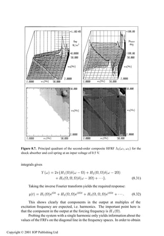

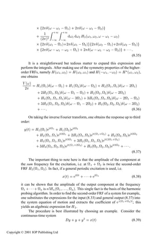

![392 The Volterra series and higher-order frequency response functions
this time with the notation.
À½ and À¾ for this system can be evaluated by exactly the same procedure
as used on the previous example. The results are
½
À½ ´ µ
Ñ ¾ · · (8.50)
À¾ ´ ½ ¾ µ ¾ À½ ´ ½ µÀ½ ´ ¾ µÀ½ ´ ½ · ¾ µ (8.51)
Note that the constant ¾ multiplies the whole expression for À ¾ , so that if
the square-law term is absent from the equation of motion, À ¾ vanishes. This
reflects a quite general property of the Volterra series; if all nonlinear terms in
the equation of motion for a system are odd powers of Ü or Ý , then the associated
Volterra series has no even-order kernels. As a consequence it will possess no
even-order kernel transforms.
In order to obtain À ¿ , the required probing expressions are
ܴص ÜÔ ´Øµ
¿ ½ Ø· ¾ Ø· ¿ Ø (8.52)
and
ݴص Ô
Ý¿ ´Øµ À½ ´ ½ µ ½ Ø · À½ ´ ¾ µ ¾ Ø · À½ ´ ¿ µ ¿ Ø
· ¾À¾´ ½ ¾µ ´ ½ · ¾ µØ · ¾À¾ ´ ½ ¿ µ ´ ½ · ¿ µØ
· ¾À¾´ ¾ ¿µ ´ ¾ · ¿ µØ · À¿ ´ ½ ¾ ¿ µ ´ ½ · ¾ · ¿ µØ (8.53)
which are sufficiently general to obtain À ¿ for any system. Substituting into the
Duffing equation and extracting the coefficient of ´ ½ · ¾ · ¿ µØ yields
À¿ ´ ½ ¾ ¿µ ½ À½ ´ ½ · ¾ · ¿ µ
¢ ¾´À½ ´ ½ µÀ¾ ´ ¾ ¿ µ · À½ ´ ¾ µÀ¾ ´ ¿ ½µ
· À½ ´ ¿ µÀ¾ ´ ½ ¾ µµ
· ¿ À½ ´ ½ µÀ½ ´ ¾ µÀ½ ´ ¿ µ (8.54)
A discussion of the interpretation of these functions is deferred until a little later.
It is property of many systems that all higher-order FRFs can be expressed
in terms of À½ for the system. The exact form of the expression will depend on
the particular system.
The harmonic probing algorithm has been established for continuous-time
systems, i.e. those whose evolution is governed by differential equations of
motion. The NARMAX models discussed in chapter 6 are difference equations so
the probing algorithm requires a little modification as in [32] and [256]. Consider
the difference equation analogue of equation (8.39):
Ý · Ý · ݾ ܴص (8.55)
where is the backward shift operator, defined by Ý ´Øµ Ý´Ø ½µ.
(Throughout this chapter it is assumed, except where indicated, that the sampling
Copyright © 2001 IOP Publishing Ltd](https://image.slidesharecdn.com/72268096-non-linearity-in-structural-dynamics-detection-identification-and-modelling-copy-120717010202-phpapp02/85/72268096-non-linearity-in-structural-dynamics-detection-identification-and-modelling-copy-408-320.jpg)
![Harmonic probing of the Volterra series 393
interval for a discrete-time system is scaled to unity. This yields a unit sampling
frequency and Nyquist frequency of 0.5.) In the usual notation for difference
equations, (8.55) becomes
Ý ½ · Ý · ݾ Ü (8.56)
However, the form containing allows the most direct comparison with
the continuous-time case. It is clear from the previous argument that the only
differences for harmonic probing of discrete-time systems will be generated by
the fact that the operator has a different action on functions Ø to the operator
3
. This action is very simple to compute, as shown in chapter 1 ,
Ø ´Ø ½µ ¡ Ø (8.57)
It is now clear that one can carry out the harmonic probing algorithm for
(8.55) exactly as for the continuous-time (8.39); the only difference will be that
the operator will generate a multiplier wherever generated a factor .
As a consequence À ½ and À¾ for (8.55) are easily computed.
½
À½ ´ µ ·½ (8.58)
À¾ ´ ½ ¾ µ
À½ ´ ½ µÀ½ ´ ¾ µ À ´ µÀ ´ µÀ ´ · µ
´ · µ·½
½ ¾
½ ½ ½ ½ ½ ½ ¾ (8.59)
Note that the form of À ¾ as a function of À ½ is identical to that for the
continuous-time system.
It is possible at this point to make a quite general statement. Given
a continuous-time system with linear or nonlinear equation of motion
´ Ý Üµ ¼ and HFRFs ÀÒ ´ ½ Ò µ, Ò ½ ½, the corresponding
discrete-time system ´ Ý Üµ ¼ has HFRFs ÀÒ ´ ½ Òµ
ÀÒ ´ ½ Ò µ, Ò ½ ½. Further the functional relationships
between the ÀÒ and À½ will be identical in both cases.
The system in equation (8.56) is not an NARMAX system as it is a nonlinear
function of the most recent sampled value Ý . As discussed in chapter 6, an
NARMAX, or more strictly NARX, model has the general form
Ý ´Ý ½ Ý ÒÝ Ü ½ Ü ÒÜ µ (8.60)
with appropriate noise modelling if necessary.
The relevant existence theorems obtained in [161, 162] show that this form
is general enough to represent almost all input–output systems.
¿ It is amusing to note that this action follows from the fact that as an operator equation;
as Ø is an eigenfunction of with eigenvalue , it is also an eigenfunction of with eigenvalue
.
Copyright © 2001 IOP Publishing Ltd](https://image.slidesharecdn.com/72268096-non-linearity-in-structural-dynamics-detection-identification-and-modelling-copy-120717010202-phpapp02/85/72268096-non-linearity-in-structural-dynamics-detection-identification-and-modelling-copy-409-320.jpg)
![394 The Volterra series and higher-order frequency response functions
8.4 Validation and interpretation of the higher-order FRFs
In order to justify studying the higher-order FRFs it is necessary to show that
they contain useful information about whatever system is under examination. In
fact, as time- and frequency-domain representations are completely equivalent,
the higher-order FRFs contain all system information; later in this section it is
demonstrated that important facts can be conveyed in a very direct and visible
way.
Before discussing matters of interpretation it is important to address the
question of uniqueness of the higher-order FRFs as it is critical to any analysis
that the non-uniqueness of the time-domain NARMAX representation of a system
does not affect the frequency-domain representation.
The first thing which must be established is the correspondence between
the FRFs of the continuous system and the FRFs of the discrete approximations.
Consider the Duffing oscillator of equation (8.49), a discrete-time representation
for this system could be obtained by adopting discrete approximations to the
derivatives. The coarsest approximation available is the backward-difference
approximation
Ý
Ý Ý ½ (8.61)
¡Ø
Ý ·½ ¾Ý · Ý ½
Ý
¡Ø¾
(8.62)
which gives the discrete-time representation
¾Ñ · ¡Ø · ¡Ø¾ Ñ
Ý Ý ½ Ý
Ñ · ¡Ø Ñ · ¡Ø ¾
¾ ¾ ¾
Ñ ¾ ¡Ø¡Ø ݾ ½ Ñ ¿ ¡Ø¡Ø Ý¿ ½ · Ñ ¡Ø ¡Ø Ü ½
· · ·
(8.63)
In fact, because this is based on the coarse approximations (8.61) and
(8.62), it does not yield good representations of the higher-order FRFs. In order
to demonstrate accurate FRFs from a NARX model, the following numerical
simulation was carried out. A fourth-order Runge–Kutta scheme [209], was used
to obtain the response of the system (8.49) under excitation by a Gaussian noise
sequence ܴص with rms 10.0 and frequency range 0–90 Hz. The coefficient values
adopted were: Ñ ½, ¾¼, ½¼ , ¾ ½¼ , ¿ ¢ ½¼ . This system
has a resonant frequency of Ö rad s ½ or Ö ¾ Ö
½ Hz. The data
were generated with a sampling interval of 0.005 s, giving a Nyquist frequency of
100 Hz.
A NARX model was fitted to 1000 points of the resulting discrete Ü and
Ý data using the estimation and validation methods described in the previous
Copyright © 2001 IOP Publishing Ltd](https://image.slidesharecdn.com/72268096-non-linearity-in-structural-dynamics-detection-identification-and-modelling-copy-120717010202-phpapp02/85/72268096-non-linearity-in-structural-dynamics-detection-identification-and-modelling-copy-410-320.jpg)


![Validation and interpretation of the higher-order FRFs 403
and a similar analysis for (8.73) gives
½
À½ ¿µ´ µ
´ ½· « ·Ç´«¾ µ À½ ½µ ´ µ·Ç´«¾ µ
´
½ «
(8.75)
Note that by retaining Ò terms in the binomial expansion, the model
Ý Ü ½ · «Ü ¾ · ¡ ¡ ¡ · «Ò ½ Ü Ò (8.76)
is obtained which is equivalent to (8.71) up to Ç´« Ò µ. As a result, the system
(8.71) can be represented with arbitrary accuracy by the binomial expansion if
Ò is large enough. However, note that one representation has only three model
terms while the other has Ò with Ò possibly large. This serves to illustrate why
it is important to correctly detect the model structure or which terms are in the
model in order to yield a parsimonious model [32].
One must be careful not to regard these simple arguments as generating
a general principle; however, it would seem likely that equivalence of two
NARX models up to a given order of accuracy would imply equivalence of the
corresponding HFRFs up to the same order of accuracy. This is easy to establish
in the case of a general linear system by an extension of the previous argument.
The various cases discussed earlier exhaust all possibilities for obtaining
different NARX representations of a given system.
This discussion is simply intended as an argument that all NARX models
which are equivalent in the sense that they furnish a discrete approximation to
a continuous system will have higher-order FRFs which not only approximate
to each other but also to those of the underlying continuous system. It does
not constitute a rigorous proof in any sense; however, it is difficult to imagine
a situation under which this condition would not hold.
Having established some confidence in their reliability, the interpretation of
the higher-order FRFs can be discussed. The Duffing oscillator system (8.49)
serves well as an illustration. The magnitude and phase of the expression (8.50)
for À½ ´ µ À½ ´¾ µ is given in figures 8.10(a) and (b) on the frequency interval
0–100 Hz. The interpretation of these figures, traditionally given together and
universally called the Bode plot, has been described in earlier chapters, notably
chapter 1. The peak in the magnitude at Ö ½ Hz shows that for
this frequency of excitation the amplitude of the linear part of the response Ý ½ ´Øµ
is a maximum. The Bode plot thus allows the immediate identification of those
excitation frequencies at which the vibration level of the system is likely to be
high.
Interpretation of the second-order FRF is also straightforward. The
magnitude and phase of À ¾ for the Duffing system given earlier are given in
figures 8.11(a) and (b) as surfaces, or in figures 8.12(a) and (b) as contour maps,
over the ´ ½ ¾ µ ´ ¾ ½ ¾ ¾ µ plane. The frequency ranges for the plot are the same
as for À½ in figure 8.10. A number of ridges are observed. These are in direct
correspondence with the peak in À ½ as follows. According to equation (8.51),
Copyright © 2001 IOP Publishing Ltd](https://image.slidesharecdn.com/72268096-non-linearity-in-structural-dynamics-detection-identification-and-modelling-copy-120717010202-phpapp02/85/72268096-non-linearity-in-structural-dynamics-detection-identification-and-modelling-copy-419-320.jpg)
![404 The Volterra series and higher-order frequency response functions
À¾ is a constant multiple of À½ ´ ½ µÀ½ ´ ¾ µÀ½ ´ ½ · ¾ µ. As a consequence À¾
possesses local maxima at positions where the À ½ factors have local maxima.
Consequently there are two ridges in the À ¾ surface corresponding to the lines
½ Ö ¾ Ö and ¾ Ö . These are along lines parallel to the frequency
axes. In addition, À ¾ has local maxima generated by the À ½ ´ ½ · ¾ µ factor
along the line ½ · ¾ Ö . This ridge has an important implication; it indicates
that one can expect a maximum in the second-order output Ý ¾ ´Øµ if the system is
excited by two sinusoids whose sum frequency is the linear resonant frequency.
This shows clearly why estimation of a transfer function by linear methods is
inadequate for nonlinear systems; such a transfer function would usually indicate
a maximum in the output for a harmonic excitation close to the linear resonant
frequency. However, it would fail to predict that one could excite a large nonlinear
component in the output by exciting at
ÖØ ÖØ ÖØ
¾Ö ; this is a consequence of the
trivial decomposition ¾ ¾ ¾ · ¾ which means that the signal can be
regarded as a ‘two-tone’ input with a sum frequency at the linear resonance Ö .
The importance of the second-order FRF is now clear. It reveals those pairs of
excitation frequencies which will conspire to produce large levels of vibration as
a result of second-order nonlinear effects.
The interpretation of À ¿ for the system is very similar. Consideration of
equation (8.54) shows that for a three-tone input of the form (8.52) one should
expect maxima in the third-order output Ý ¿ ´Øµ if the following conditions are
satisfied: ½ Ö, ¾ Ö, ¿ Ö, ½ · ¾ Ö, ¾ · ¿ Ö, ¿ · ½ Ö,
½ · ¾· ¿ Ö . The presence of these ‘combination resonances’ would be
indicated by the presence of ridges in the À ¿ surface. Although figures 8.13 and
8.14 only show the ‘projections’ of À ¿ over the ´ ½ ¾ µ-plane, they are sufficient
to indicate the presence of the ‘combination resonances’ ½ Ö, ¾ Ö,
½ · ¾ Ö ,¾ ½ Ö ,¾ ½· ¾ Ö . It is clear that the local maximum
distributions become more and more complex as the order of the HFRF increases.
These arguments show that the higher-order FRFs provide directly visible
information about the possible excitation of large nonlinear vibrations through
the cooperation of certain frequencies.
8.5 An application to wave forces
The power of the NARX and higher-order FRF approaches can be demonstrated
by the following example used in chapter 6 where force and velocity data were
obtained from a circular cylinder placed in a planar oscillating fluid flow in a large
U-tube [199]. The standard means of predicting forces on cylinders used by the
offshore industry is to use Morison’s equation (6.121) which expresses the force
as a simple nonlinear function of the instantaneous flow velocity and acceleration.
For one particular frequency of flow oscillation, Morison’s equation gave the force
prediction shown in figure 8.16(a) compared with the measured force. Morison’s
equation is inadequate at representing the higher-frequency components of the
Copyright © 2001 IOP Publishing Ltd](https://image.slidesharecdn.com/72268096-non-linearity-in-structural-dynamics-detection-identification-and-modelling-copy-120717010202-phpapp02/85/72268096-non-linearity-in-structural-dynamics-detection-identification-and-modelling-copy-420-320.jpg)
![FRFs and Hilbert transforms: sine excitation 405
force. The model inadequacy is shown clearly by the correlation-based validity
tests (section 6.8.3) in figure 8.17(b) 4.
A NARX fit to the force–velocity data gave the model prediction shown in
figure 8.17(a). This model also passes the correlation tests (figure 8.17(b)).
A similar analysis has been carried out on fluid-loading data encompassing
a broad range of flow conditions ranging from U-tube data to that from a
unidirectional wave in a large flume to data from a random directional sea. In all
cases, the NARX analysis produced a better model than Morison’s equation [276].
Unfortunately the model structures varied. In order to examine the possibility
that this was simply due to the non-uniqueness of the NARX representations,
the higher-order FRFs were obtained by harmonic probing. The results were
very interesting, as an example, À ¿ for the U-tube data of figure 8.17 is given
in figure 8.18. The pronounced ridges were shown to appear in the third-order
FRFs for all of the flow conditions examined; this is in direct contradiction to
Morison’s equation which forces a constant À ¿ .
The higher-order FRFs can often throw light onto a problem in this way;
the direct visualization of the system properties which they provide is appealing.
They have actually been used in wave loading studies for some time now;
however, the computational burden imposed by traditional methods of estimation
has prohibited the use of functions higher than second order [85]
8.6 FRFs and Hilbert transforms: sine excitation
8.6.1 The FRF
It was shown earlier that the Volterra series provides a convenient means for
calculating the nonlinear system response to a single harmonic; this forms the
basis of the harmonic probing method. It is only slightly more complicated to
calculate the response to multiple harmonics. The benefit is that one can then
determine the response to a sinusoid and this, in turn, will allow us to develop an
expression for the stepped-sine FRF of the system. Suppose the excitation is a
two-tone signal
ܴص ª Ø· ª Ø (8.77)
which translates into the frequency domain as
´ µ ¾ Æ´ ª µ · Æ´ ª µ (8.78)
Substituting this into (8.16)–(8.18) and thence into (8.15) leads, after a long
but straightforward calculation, to
ݴص À ´ª µ ª Ø · À ´ª µ ª Ø · ¾ À ´ª ª µ ¾ ª Ø
½ ½ ¾
Of course, with enough parameters, one can fit a model to an arbitrary level of accuracy on a given
estimation set of data. The modeller should always carry out appropriate levels of model validity
testing in order to ensure that the model is genuine and does not simply represent an isolated data set.
This is particularly pressing in the situation where one might abandon a physical model like Morison’s
equation in favour of a non-physical model on the grounds of model accuracy.
Copyright © 2001 IOP Publishing Ltd](https://image.slidesharecdn.com/72268096-non-linearity-in-structural-dynamics-detection-identification-and-modelling-copy-120717010202-phpapp02/85/72268096-non-linearity-in-structural-dynamics-detection-identification-and-modelling-copy-421-320.jpg)


![410 The Volterra series and higher-order frequency response functions
(adopting lower-case from now on) or
À¿ ´ µ ¿ À½ ´ µ¿ À½£ ´ µ (8.88)
Harmonic balance gives for (8.49)
½
À´ ½ ¾ ¿ µ À½ ´ ½ · ¾ · ¿ · · µ
¢ ´ ¿ ¿ ¿ À¿´ ½ ¾ ¿µÀ½ ´ µÀ½ ´ µ
· À¿ ´ ½ ¾ µÀ½ ´ ¿ µÀ½ ´ µ
· À¿ ´ ½ ¿ µÀ½ ´ ¾ µÀ½ ´ µ · À¿ ´ ¾ ¿ µÀ½ ´ ½ µÀ½ ´ µ
· À¿ ´ ½ ¾ µÀ½ ´ ¿ µÀ½ ´ µ · À¿ ´ ½ ¿ µÀ½ ´ ¾ µÀ½ ´ µ
· À¿ ´ ¾ ¿ µÀ½ ´ ½ µÀ½ ´ µ · À¿ ´ ½ µÀ½ ´ ¾ µÀ ½ ´ ¿µ
· À¿ ´ ¾ µÀ½ ´ ½ µÀ½ ´ ¿ µ · À¿ ´ ¿ µÀ½ ´ ½ µÀ ½ ´ ¾µ µ
(8.89)
and thence
À´ ¿ ¾ £ ¿ £ ¾
µ ½¼ ¿ ´¿À½ ´ µ À½ ´ µ · À½ ´ µ À½ ´ µ
· À½ ´ µ À½ ´ µ¾ À½ ´¿ µµ
£ (8.90)
Substituting (8.90) and (8.88) into (8.86) gives the FRF up to Ç´ µ
¿ ¾ ¿
£× ´ªµ À½ ´ªµ ¿ À½ ´ µ¿ À½ ´ µ · ½ ¿ ´¿À½ ´ µ À½ ´ µ¿
£ ¾ £
· À½ ´ µ À½ ´ µ¾ · À½ ´ µ À½ ´ µ¾ À½ ´¿ µµ · Ç´ µ (8.91)
£ £
(Amongst other places, this equation has been discussed in [236], where it
was used to draw some conclusions regarding the amplitude dependence of the
stepped-sine composite FRF.)
In order to illustrate these expressions, the system
Ý · ¾¼Ý · ½¼ Ý · ¢ ½¼ Ý¿ Ó×´ ص (8.92)
was chosen. Figure 8.19 shows the FRF magnitude plots obtained from (8.91)
for ¼ ¼½ (near linear), ¼ and ¼ . At the higher amplitudes,
the expected FRF distortion is obtained, namely the resonant frequency shifts
up and the magnitude at resonance falls. Figure 8.20 shows the corresponding
Nyquist plots. (Note the unequal scales in the Real and Imaginary axes; the plots
are effectively circular.) Figure 8.21 shows the Ç´ µ FRF compared with the
‘exact’ result from numerical simulation. There is a small degree of error near
resonance which is the result of premature truncation of the Volterra series.
Copyright © 2001 IOP Publishing Ltd](https://image.slidesharecdn.com/72268096-non-linearity-in-structural-dynamics-detection-identification-and-modelling-copy-120717010202-phpapp02/85/72268096-non-linearity-in-structural-dynamics-detection-identification-and-modelling-copy-426-320.jpg)


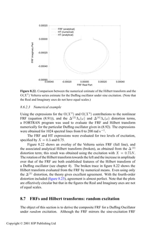
![FRFs and Hilbert transforms: random excitation 417
0.00020
FRF (analytical)
HT (numerical)
HT (analytical)
0.00000
FRF Imaginary Part
-0.00020
-0.00040
-0.00060
-0.00040 -0.00020 0.00000 0.00020 0.00040
FRF Real Part
Figure 8.23. Comparison between the numerical estimate of the Hilbert transform and the
Ç´ µ Volterra series estimate for the Duffing oscillator under sine excitation. (Note that
the Real and Imaginary axes do not have equal scales.)
in many respects, there are important differences. This section is this book’s
only real foray into the realm of random vibration. If the reader would like to
study the subject in more depth, [198] is an excellent example of an introductory
textbook. A considerably more advanced treatment can be found in [52], which
treats nonlinear random vibration amongst other topics.
There have been a number of related calculations over the years. The
simplest method of approximating an FRF for a nonlinear system is based on
equivalent linearization [54]. This approach estimates the parameters of the linear
system which is closest (in a statistical sense) to the original nonlinear system.
The FRF of the linearized system is computed. In [75], statistical linearization
was combined with perturbation analysis [68], in order to calculate the spectral
response of a Duffing oscillator to white noise excitation. (This is equivalent
to the FRF calculation up to a multiplicative constant.) It was shown that the
FRF exhibits a secondary peak at three times the natural frequency, a result
which is unavailable from statistical linearization alone. An approach based on
perturbation theory alone is described in [147] and the calculation is carried to
first order in the perturbation parameter. A number of studies of spectra have
appeared based on the use of the Fokker–Planck–Kolmogorov equation (FPK)
[55, 15, 137, 138, 284]. The latter two references actually examine the Duffing
oscillator system which is studied in the current work. Good representations of
the spectra were obtained; however, to the order of approximation pursued, the
approach was unable to explain the presence of the secondary peak described
Copyright © 2001 IOP Publishing Ltd](https://image.slidesharecdn.com/72268096-non-linearity-in-structural-dynamics-detection-identification-and-modelling-copy-120717010202-phpapp02/85/72268096-non-linearity-in-structural-dynamics-detection-identification-and-modelling-copy-433-320.jpg)
![418 The Volterra series and higher-order frequency response functions
earlier. An interesting approach to approximating the spectral response of a
Duffing oscillator is adopted in [184]. There, the expected response of an
equivalent linear system was calculated where the natural frequency of the
linear system was a random variable. The results compared favourably with
numerical simulation, but the secondary peak could not be obtained. The Volterra
series approach given here has been applied in [53] and [250], amongst others;
however, the calculation was not carried far enough to allow a description of
FRF distortions or the occurrence of the secondary peak. Using a Volterra
series approach also allows the definition of higher(polynomial)-order equivalent
systems, for example, the method of statistical quadratization is discussed in [78].
8.7.1 Volterra system response to a white Gaussian input
The problem of nonlinear system response to a generic random input is
completely intractable. In order to make progress, it is usually assumed that
the noise is white Gaussian. The power spectrum of such an input is constant
over all frequencies and, as a consequence, Gaussian white noise is a physically
unrealizable signal since it has infinite power. In practice, Gaussian white
noise is approximated by Gaussian random processes that have sufficiently broad
frequency bandwidth for the application of interest.
The definition of the FRF of a linear system based on the input/output
cross-spectrum, Ë ÝÜ ´ µ, and input auto-spectrum, Ë ÜÜ ´ µ, is well known (and
is repeated here for convenience)
ËÝÜ´ µ
À´ µ À½ ´ µ (8.114)
ËÜÜ´ µ
The composite FRF, £ Ö ´ µ, of a nonlinear system under random excitation
is defined similarly
ËÝÜ ´ µ
£Ö ´ µ (8.115)
ËÜÜ´ µ
The term composite FRF is used again because £ Ö ´ µ, for a nonlinear
system, will not in general be equal to À ½ ´ µ but will receive contributions from
all ÀÒ . It will be shown that random excitation leads to a different composite
FRF than sine excitation, hence the identifying subscript. The FRF also depends
on the power spectral density of the input. However, £ Ö ´ µ tends to the linear
FRF as the power spectral density of the excitation tends to zero.
In order to obtain a more detailed expression for £ Ö ´ µ, an expression for
ËÝÜ ´ µ must be derived. Using the Volterra series representation given in (8.3)
results in the expression
Ëݽ Ü ´ µ · Ëݾ Ü ´ µ · ¡ ¡ ¡ · ËÝÒÜ ´ µ · ¡ ¡ ¡
£Ö´ µ (8.116)
ËÜÜ ´ µ
£Ö ´ µ will be approximated here by obtaining expressions for the various cross-
spectra between the input and the individual output components. First, consider
Copyright © 2001 IOP Publishing Ltd](https://image.slidesharecdn.com/72268096-non-linearity-in-structural-dynamics-detection-identification-and-modelling-copy-120717010202-phpapp02/85/72268096-non-linearity-in-structural-dynamics-detection-identification-and-modelling-copy-434-320.jpg)

![420 The Volterra series and higher-order frequency response functions
It can be shown [158] that for zero-mean Gaussian variables Ü ½ ܾ
ÜÒ
ܽ ܾ ÜÒ ¼ (8.123)
if Ò is odd and if Ò is even
ܽ ܾ ÜÒ ÜÜ (8.124)
ÈÉ
where means the sum of the products of Ü Ü , the pairs Ü Ü being taken
from ܽ ܾ ÜÒ in all the possible distinct ways.
It follows from (8.123) that all cross-correlation functions, and hence all
cross-spectra, between the input and the even-order output components will be
zero, i.e. ËÝ¾Ò Ü ´ µ Ý¾Ò Ü ´ µ ¼, Ò.
Moving on to the Ë Ý¿ Ü ´ µ term, this is given by
·½ ·½ ·½
Ý¿ Ü ´ µ ½ ¾ ¿ ¿´ ½ ¾ ¿µ
½ ½ ½
¢ Ü´Ø ½ µÜ´Ø ¾ µÜ´Ø ¿ µÜ´Ø µ (8.125)
From (8.124) the expected value of the product of inputs, i.e. the fourth-order
moment of the input, reduces to the following product of second-order moments,
Ü´Ø ½ µÜ´Ø ¾ µÜ´Ø ¿ µÜ´Ø µ
Ü´Ø ½ µÜ´Ø ¾ µ Ü´Ø ¿ µÜ´Ø µ
· Ü´Ø ½ µÜ´Ø ¿ µ Ü´Ø ¾ µÜ´Ø µ
· Ü´Ø ½ µÜ´Ø µ Ü´Ø ¾ µÜ´Ø ¿ µ (8.126)
Using this equation and taking advantage of the symmetry of the Volterra
kernels leads to
·½ ·½ ·½
Ý¿ Ü ´ µ ¿ ½ ¾ ¿ ¿´ ½ ¾ ¿µ
½ ½ ½
¢ Ü´Ø ½ µÜ´Ø ¾ µ Ü´Ø ¿ µÜ´Ø µ
·½ ·½ ·½
¿ ½ ¾ ¿ ¿´ ½ ¾ ¿µ
½ ½ ½
¢ ÜÜ ´ ¾ ½ µ ÜÜ ´ ¿ µ (8.127)
Fourier transforming this equation and manipulating the result eventually
yields
¿ËÜÜ´ µ ·½
ËÝ¿ Ü ´ µ
¾ ½ À¿ ´ ½ ½ µËÜÜ´ ½ µ (8.128)
½
This result is already available in the literature [25]. Its presence here is
justified by the fact that the derivation of the general term is a simple modification.
Copyright © 2001 IOP Publishing Ltd](https://image.slidesharecdn.com/72268096-non-linearity-in-structural-dynamics-detection-identification-and-modelling-copy-120717010202-phpapp02/85/72268096-non-linearity-in-structural-dynamics-detection-identification-and-modelling-copy-436-320.jpg)

![422 The Volterra series and higher-order frequency response functions
· À½ ´ ½ · ¾ · µ · À½ ´ ½ ¾ · µ
¿ ¿¾
À ´ µ¾ À½ ´ ½ µ ¾ À½ ´ ¾ µ ¾ ¾À½ ´ µ · À½ ´ ½ µ · À½ ´ ½µ
½¼ ½
· À½ ´ ¾ µ · À½ ´ ¾ µ · À½ ´ ½ · ¾ · µ · À½ ´ ½ ¾ · µ
· À½ ´ ½ · ¾ · µ · À½ ´ ½ ¾ · µ (8.133)
Ë ¿Ü´ µ
So only one integral needs to be evaluated for ËÝÜÜ ´ µ compared to nine for
ËÝ Ü ´ µ
ËÜÜ ´ µ .
Ë ¿Ü´ µ
Substituting (8.132) into the ËÝÜÜ ´ µ term of (8.131) gives
ËÝ¿ Ü ´ µ À ¾ ·½
ËÜÜ ´ µ
¿È ¿¾ ½ ´ µ ½ À½ ´ ½ µ ¾ (8.134)
½
This integral may be found in standard tables of integrals used for the
calculation of mean-square response, e.g. [198]. However, the analysis is
instructive and it will allow the definition of notation for the integrals which
follow.
Consider the common expression for the linear FRF (8.97). In terms of this,
¾
the integral in (8.134), À ½ ´ ½ µ may be written
½
À½ ´ ½ µ ¾
Ѿ ´ ½ Ô½ µ´ ½ Ô¾ µ´ ½ Ô£ µ´ ½ Ô£ µ
(8.135)
½](https://image.slidesharecdn.com/72268096-non-linearity-in-structural-dynamics-detection-identification-and-modelling-copy-120717010202-phpapp02/85/72268096-non-linearity-in-structural-dynamics-detection-identification-and-modelling-copy-438-320.jpg)


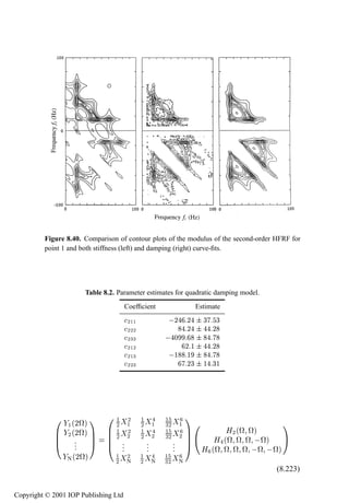


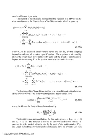


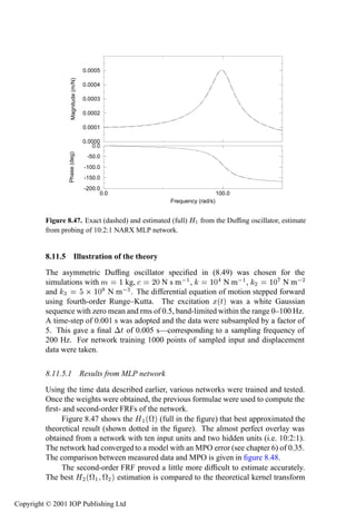


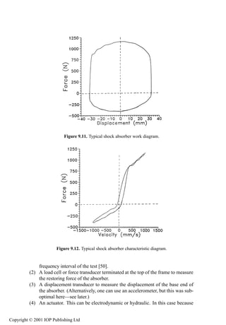


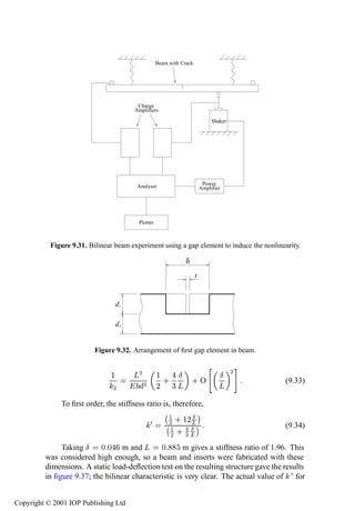


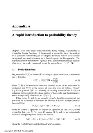


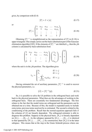


More Related Content


Similar to 72268096 non-linearity-in-structural-dynamics-detection-identification-and-modelling-copy (20)
![[Ashish tewari] modern_control_design_with_matlab_(book_fi.org)](https://cdn.slidesharecdn.com/ss_thumbnails/ashishtewarimoderncontroldesignwithmatlabbookfi-org-120829235237-phpapp01-thumbnail.jpg?width=560&fit=bounds)


72268096 non-linearity-in-structural-dynamics-detection-identification-and-modelling-copy
- 1. NONLINEARITY IN STRUCTURAL DYNAMICS Detection, Identification and Modelling K Worden and G R Tomlinson University of Sheffield, UK Institute of Physics Publishing Bristol and Philadelphia Copyright © 2001 IOP Publishing Ltd
- 2. IOP Publishing Ltd 2001 c All rights reserved. No part of this publication may be reproduced, stored in a retrieval system or transmitted in any form or by any means, electronic, mechanical, photocopying, recording or otherwise, without the prior permission of the publisher. Multiple copying is permitted in accordance with the terms of licences issued by the Copyright Licensing Agency under the terms of its agreement with the Committee of Vice-Chancellors and Principals. British Library Cataloguing-in-Publication Data A catalogue record for this book is available from the British Library. ISBN 0 7503 0356 5 Library of Congress Cataloging-in-Publication Data are available Commissioning Editor: James Revill Production Editor: Simon Laurenson Production Control: Sarah Plenty Cover Design: Victoria Le Billon Marketing Executive: Colin Fenton Published by Institute of Physics Publishing, wholly owned by The Institute of Physics, London Institute of Physics Publishing, Dirac House, Temple Back, Bristol BS1 6BE, UK US Office: Institute of Physics Publishing, The Public Ledger Building, Suite 1035, 150 South Independence Mall West, Philadelphia, PA 19106, USA Typeset in TEX using the IOP Bookmaker Macros Printed in the UK by J W Arrowsmith Ltd, Bristol Copyright © 2001 IOP Publishing Ltd
- 3. For Heather and Margaret Copyright © 2001 IOP Publishing Ltd
- 4. ‘As you set out for Ithaka hope your road is a long one, full of adventure, full of discovery. Laistrygonians, Cyclops, angry Poseidon—don’t be afraid of them: You’ll never find things like that in your way as long as you keep your thoughts raised high, as long as a rare sensation touches your body and spirit. Laistrygonians, Cyclops, wild Poseidon—you won’t encounter them unless you bring them along inside your soul, Unless your soul sets them up in front of you.’ C P Cavafy, ‘Ithaka’ Copyright © 2001 IOP Publishing Ltd
- 5. Contents Preface xv 1 Linear systems 1 1.1 Continuous-time models: time domain 1 1.2 Continuous-time models: frequency domain 10 1.3 Impulse response 13 1.4 Discrete-time models: time domain 17 1.5 Classification of difference equations 21 1.5.1 Auto-regressive (AR) models 21 1.5.2 Moving-average (MA) models 21 1.5.3 Auto-regressive moving-average (ARMA) models 22 1.6 Discrete-time models: frequency domain 22 1.7 Multi-degree-of-freedom (MDOF) systems 23 1.8 Modal analysis 29 1.8.1 Free, undamped motion 29 1.8.2 Free, damped motion 35 1.8.3 Forced, damped motion 37 2 From linear to nonlinear 41 2.1 Introduction 41 2.2 Symptoms of nonlinearity 41 2.2.1 Definition of linearity—the principle of superposition 41 2.2.2 Harmonic distortion 46 2.2.3 Homogeneity and FRF distortion 49 2.2.4 Reciprocity 51 2.3 Common types of nonlinearity 52 2.3.1 Cubic stiffness 52 2.3.2 Bilinear stiffness or damping 55 2.3.3 Piecewise linear stiffness 55 2.3.4 Nonlinear damping 56 2.3.5 Coulomb friction 57 2.4 Nonlinearity in the measurement chain 57 2.4.1 Misalignment 58 Copyright © 2001 IOP Publishing Ltd
- 6. viii Contents 2.4.2 Vibration exciter problems 59 2.5 Two classical means of indicating nonlinearity 59 2.5.1 Use of FRF inspections—Nyquist plot distortions 60 2.5.2 Coherence function 62 2.6 Use of different types of excitation 65 2.6.1 Steady-state sine excitation 66 2.6.2 Impact excitation 67 2.6.3 Chirp excitation 68 2.6.4 Random excitation 68 2.6.5 Conclusions 69 2.7 FRF estimators 69 2.8 Equivalent linearization 72 2.8.1 Theory 72 2.8.2 Application to Duffing’s equation 76 2.8.3 Experimental approach 78 3 FRFs of nonlinear systems 81 3.1 Introduction 81 3.2 Harmonic balance 81 3.3 Harmonic generation in nonlinear systems 88 3.4 Sum and difference frequencies 90 3.5 Harmonic balance revisited 91 3.6 Nonlinear damping 93 3.7 Two systems of particular interest 95 3.7.1 Quadratic stiffness 95 3.7.2 Bilinear stiffness 98 3.8 Application of harmonic balance to an aircraft component ground vibration test 101 3.9 Alternative FRF representations 105 3.9.1 Nyquist plot: linear system 105 3.9.2 Nyquist plot: velocity-squared damping 107 3.9.3 Nyquist plot: Coulomb friction 108 3.9.4 Carpet plots 109 3.10 Inverse FRFs 111 3.11 MDOF systems 112 3.12 Decay envelopes 122 3.12.1 The method of slowly varying amplitude and phase 122 3.12.2 Linear damping 124 3.12.3 Coulomb friction 125 3.13 Summary 125 Copyright © 2001 IOP Publishing Ltd
- 7. Contents ix 4 The Hilbert transform—a practical approach 127 4.1 Introduction 127 4.2 Basis of the method 128 4.2.1 A relationship between real and imaginary parts of the FRF128 4.2.2 A relationship between modulus and phase 132 4.3 Computation 132 4.3.1 The direct method 133 4.3.2 Correction methods for truncated data 135 4.3.3 Fourier method 1 142 4.3.4 Fourier method 2 149 4.3.5 Case study of the application of Fourier method 2 153 4.4 Detection of nonlinearity 156 4.4.1 Hardening cubic stiffness 160 4.4.2 Softening cubic stiffness 161 4.4.3 Quadratic damping 161 4.4.4 Coulomb friction 163 4.5 Choice of excitation 165 4.6 Indicator functions 168 4.6.1 NPR: non-causal power ratio 168 4.6.2 Corehence 170 4.6.3 Spectral moments 170 4.7 Measurement of apparent damping 173 4.8 Identification of nonlinear systems 175 4.8.1 FREEVIB 180 4.8.2 FORCEVIB 189 4.9 Principal component analysis (PCA) 190 5 The Hilbert transform—a complex analytical approach 202 5.1 Introduction 202 5.2 Hilbert transforms from complex analysis 202 5.3 Titchmarsh’s theorem 205 5.4 Correcting for bad asymptotic behaviour 207 5.4.1 Simple examples 209 5.4.2 An example of engineering interest 211 5.5 Fourier transform conventions 215 5.6 Hysteretic damping models 217 5.7 The Hilbert transform of a simple pole 223 5.8 Hilbert transforms without truncation errors 224 5.9 Summary 228 6 System identification—discrete time 230 6.1 Introduction 230 6.2 Linear discrete-time models 232 6.3 Simple least-squares methods 233 6.3.1 Parameter estimation 233 Copyright © 2001 IOP Publishing Ltd
- 8. x Contents 6.3.2 Parameter uncertainty 235 6.3.3 Structure detection 237 6.4 The effect of noise 237 6.5 Recursive least squares 242 6.6 Analysis of a time-varying linear system 246 6.7 Practical matters 249 6.7.1 Choice of input signal 249 6.7.2 Choice of output signal 251 6.7.3 Comments on sampling 252 6.7.4 The importance of scaling 253 6.8 NARMAX modelling 255 6.9 Model validity 257 6.9.1 One-step-ahead predictions 258 6.9.2 Model predicted output 258 6.9.3 Correlation tests 259 6.9.4 Chi-squared test 260 6.9.5 General remarks 260 6.10 Correlation-based indicator functions 260 6.11 Analysis of a simulated fluid loading system 261 6.12 Analysis of a real fluid loading system 273 6.13 Identification using neural networks 277 6.13.1 Introduction 277 6.13.2 A linear system 282 6.13.3 A nonlinear system 283 7 System identification—continuous time 285 7.1 Introduction 285 7.2 The Masri–Caughey method for SDOF systems 286 7.2.1 Basic theory 286 7.2.2 Interpolation procedures 290 7.2.3 Some examples 292 7.3 The Masri–Caughey method for MDOF systems 305 7.3.1 Basic theory 305 7.3.2 Some examples 310 7.4 Direct parameter estimation for SDOF systems 315 7.4.1 Basic theory 315 7.4.2 Display without interpolation 319 7.4.3 Simple test geometries 322 7.4.4 Identification of an impacting beam 325 7.4.5 Application to measured shock absorber data 334 7.5 Direct parameter estimation for MDOF systems 341 7.5.1 Basic theory 341 7.5.2 Experiment: linear system 346 7.5.3 Experiment: nonlinear system 350 Copyright © 2001 IOP Publishing Ltd
- 9. Contents xi 7.6 System identification using optimization 355 7.6.1 Application of genetic algorithms to piecewise linear and hysteretic system identification 356 7.6.2 Identification of a shock absorber model using gradient descent 367 8 The Volterra series and higher-order frequency response functions 377 8.1 The Volterra series 377 8.2 An illustrative case study: characterization of a shock absorber 380 8.3 Harmonic probing of the Volterra series 386 8.4 Validation and interpretation of the higher-order FRFs 394 8.5 An application to wave forces 404 8.6 FRFs and Hilbert transforms: sine excitation 405 8.6.1 The FRF 405 8.6.2 Hilbert transform 411 8.7 FRFs and Hilbert transforms: random excitation 416 8.7.1 Volterra system response to a white Gaussian input 418 8.7.2 Random excitation of a classical Duffing oscillator 421 8.8 Validity of the Volterra series 431 8.9 Harmonic probing for a MDOF system 434 8.10 Higher-order modal analysis: hypercurve fitting 438 8.10.1 Random excitation 440 8.10.2 Sine excitation 444 8.11 Higher-order FRFs from neural network models 450 8.11.1 The Wray–Green method 452 8.11.2 Harmonic probing of NARX models: the multi-layer perceptron 455 8.11.3 Radial basis function networks 458 8.11.4 Scaling the HFRFs 460 8.11.5 Illustration of the theory 462 8.12 The multi-input Volterra series 466 8.12.1 HFRFs for a continuous-time MIMO system 467 8.12.2 HFRFs for a discrete-time MIMO system 473 9 Experimental case studies 477 9.1 An encastr´ beam rig e 477 9.1.1 Theoretical analysis 478 9.1.2 Experimental analysis 481 9.2 An automotive shock absorber 493 9.2.1 Experimental set-up 494 9.2.2 Results 501 9.2.3 Polynomial modelling 507 9.2.4 Conclusions 510 9.3 A bilinear beam rig 511 9.3.1 Design of the bilinear beam 512 Copyright © 2001 IOP Publishing Ltd
- 10. xii Contents 9.3.2 Frequency-domain characteristics of the bilinear beam 518 9.3.3 Time-domain characteristics of the bilinear beam 523 9.3.4 Internal resonance 526 9.3.5 A neural network NARX model 530 9.4 Conclusions 531 A A rapid introduction to probability theory 533 A.1 Basic definitions 533 A.2 Random variables and distributions 534 A.3 Expected values 537 A.4 The Gaussian distribution 541 B Discontinuities in the Duffing oscillator FRF 543 C Useful theorems for the Hilbert transform 546 C.1 Real part sufficiency 546 C.2 Energy conservation 546 C.3 Commutation with differentiation 547 C.4 Orthogonality 548 C.5 Action as a filter 549 C.6 Low-pass transparency 550 D Frequency domain representations of Æ ´Øµ and ¯´Øµ 552 E Advanced least-squares techniques 554 E.1 Orthogonal least squares 554 E.2 Singular value decomposition 560 E.3 Comparison of LS methods 562 E.3.1 Normal equations 562 E.3.2 Orthogonal least squares 563 E.3.3 Singular value decomposition 563 E.3.4 Recursive least squares 563 F Neural networks 566 F.1 Biological neural networks 566 F.1.1 The biological neuron 567 F.1.2 Memory 569 F.1.3 Learning 570 F.2 The McCulloch–Pitts neuron 570 F.2.1 Boolean functions 571 F.2.2 The MCP model neuron 573 F.3 Perceptrons 579 F.3.1 The perceptron learning rule 581 F.3.2 Limitations of perceptrons 582 F.4 Multi-layer perceptrons 583 F.5 Problems with MLPs and (partial) solutions 586 F.5.1 Existence of solutions 586 Copyright © 2001 IOP Publishing Ltd
- 11. Contents xiii F.5.2 Convergence to solutions 586 F.5.3 Uniqueness of solutions 586 F.5.4 Optimal training schedules 587 F.6 Radial basis functions 587 G Gradient descent and back-propagation 590 G.1 Minimization of a function of one variable 590 G.1.1 Oscillation 591 G.1.2 Local minima 592 G.2 Minimizing a function of several variables 592 G.3 Training a neural network 595 H Properties of Chebyshev polynomials 601 H.1 Definitions and orthogonality relations 601 H.2 Recurrence relations and Clenshaw’s algorithm 602 H.3 Chebyshev coefficients for a class of simple functions 604 H.4 Least-squares analysis and Chebyshev series 605 I Integration and differentiation of measured time data 607 I.1 Time-domain integration 608 I.1.1 Low-frequency problems 608 I.1.2 High-frequency problems 614 I.2 Frequency characteristics of integration formulae 616 I.3 Frequency-domain integration 619 I.4 Differentiation of measured time data 622 I.5 Time-domain differentiation 624 I.6 Frequency-domain differentiation 626 J Volterra kernels from perturbation analysis 627 K Further results on random vibration 631 K.1 Random vibration of an asymmetric Duffing oscillator 631 K.2 Random vibrations of a simple MDOF system 633 K.2.1 The MDOF system 633 K.2.2 The pole structure of the composite FRF 634 K.2.3 Validation 636 Bibliography 641 Copyright © 2001 IOP Publishing Ltd
- 12. Preface Nonlinearity is a frequent visitor to engineering structures which can modify— sometimes catastrophically—the design behaviour of the systems. The best laid plans for a linear system will often go astray due to, amongst other things, clearances and interfacial movements in the fabricated system. There will be situations where this introduces a threat to human life; several illustrations spring to mind. First, an application in civil engineering. Many demountable structures such as grandstands at concerts and sporting events are prone to substantial structural nonlinearity as a result of looseness of joints, this creates both clearances and friction and may invalidate any linear-model-based simulations of the behaviour created by crowd movement. A second case comes from aeronautical structural dynamics; there is currently major concern in the aerospace industry regarding the possibility of limit cycle behaviour in aircraft, i.e. large amplitude coherent nonlinear motions. The implications for fatigue life are serious and it may be that the analysis of such motions is as important as standard flutter clearance calculations. There are numerous examples from the automotive industry; brake squeal is an irritating but non-life-threatening example of an undesirable effect of nonlinearity. Many automobiles have viscoelastic engine mounts which show marked nonlinear behaviour: dependence on amplitude, frequency and preload. The vast majority of engineers—from all flavours of the subject—will encounter nonlinearity at some point in their working lives, and it is therefore desirable that they at least recognize it. It is also desirable that they should understand the possible consequences and be in a position to take remedial action. The object of this book is to provide a background in techniques specific to the field of structural dynamics, although the ramifications of the theory extend beyond the boundaries of this discipline. Nonlinearity is also of importance for the diagnosis of faults in structures. In many cases, the occurrence of a fault in an initially linear structure will result in nonlinear behaviour. Another signal of the occurrence of damage is the variation with time of the system characteristics. The distinction between linear and nonlinear systems is important; nonlinear systems can exhibit extremely complex behaviour which linear systems cannot. The most spectacular examples of this occur in the literature relating to chaotic systems [248]; a system excited with a periodic driving force can exhibit an Copyright © 2001 IOP Publishing Ltd
- 13. apparently random response. In contrast, a linear system always responds to a periodic excitation with a periodic signal at the same frequency. At a less exotic level, but no less important for that, the stability theory of linear systems is well understood [207]; this is emphatically not the case for nonlinear systems. The subject of nonlinear dynamics is extremely broad and an extensive literature exists. This book is inevitably biased towards those areas which the authors are most familiar with and this of course means those areas which the authors and colleagues have conducted research in. This review is therefore as much an expression of personal prejudice and taste as anything else, and the authors would like to sincerely apologise for any inadvertent omissions. This is not to say that there are no deliberate omissions; these have good reasons which are explained here. ¯ There is no real discussion of nonlinear dynamical systems theory, i.e. phase space analysis, bifurcations of systems and vector fields, chaos. This is a subject best described by the more mathematically inclined and the reader should refer to many excellent texts. Good introductions are provided by [79] and [12]. The monograph [125] is already a classic and an overview suited to the Engineer can be found in [248]. ¯ There is no attempt to summarize many of the developments originating in control theory. The geometrical approach to nonlinearity pioneered by Brockett has led to very little concrete progress in mainstream structural dynamics beyond making rigorous some of the techniques adopted lately. The curious reader is directed to the introduction [259] or to the classic monograph [136]. Further, there is no discussion of any of the schemes based on Kalman filtering—again the feeling of the authors is that this is best left to control engineers. ¯ There is no discussion of some of the recent approaches based on spectral methods. Many of these developments can be traced back to the work of Bendat, who has summarized the background admirably in his own monograph [25] and the recent update [26]. The ‘reverse-path’ approach typified by [214] can be traced back through the recent literature survey [2]. The same authors, Adams and Allemang, have recently proposed an interesting method based on frequency response function analysis, but it is perhaps a little early to judge [3]. ¯ There is no discussion of nonlinear normal modes. Most research in structural dynamics in the past has concentrated on the effect of nonlinearity on the resonant frequencies of systems. Recently, there has been interest in estimating the effect on the modeshapes. The authors here feel that this has been dealt with perfectly adequately in the monograph [257]. There is also a useful recent review article [258]. So, what is in this book? The following is a brief outline. Chapter 1 describes the relevant background in linear structural dynamics. This is needed to understand the rest of the book. As well as describing Copyright © 2001 IOP Publishing Ltd
- 14. the fundamental measured quantities like the impulse response function (IRF) and the frequency response function (FRF) it serves to introduce notation. The backgrounds for both continuous-time systems (those based on differential equations of motion) and discrete-time (those based on difference equations) are given. The chapter begins by concentrating on single-degree- of-freedom (SDOF) linear systems and finally generalizes to those with multiple-degrees-of-freedom (MDOF) with a discussion of modal analysis. Chapter 2 gives essentially the ‘classical’ approaches to nonlinearity which have longest been within reach of structural dynamicists. This basically means approaches which can make use of standard dynamic testing equipment like frequency response analysers. Ideas like FRF distortion and coherence are discussed here. The chapter also discusses how nonlinearity can enter the measurement chain and introduces some of the more common types of nonlinearity. Finally, the idea of linearization is introduced. This chapter is not just of historical interest as most of the instrumentation commonly available commercially is still extremely restricted in its ability to deal with nonlinearity. Chapter 3. Having discussed FRF distortion, this chapter shows how to compute FRFs for nonlinear systems. It describes how each type of nonlinearity produces its own characteristic distortions and how this can lead to qualitative methods of analysis. The chapter also discusses how nonlinear systems do not follow certain behaviour patterns typical of linear systems. It shows how nonlinear systems subject to periodic forcing can respond at harmonics and combination frequencies of the forcing frequencies. The chapter concludes with an analysis of IRF distortion. Chapter 4 introduces more modern methods of analysis, in particular those which cannot be implemented on conventional instrumentation. The subject of this chapter is the Hilbert transform. This versatile technique can not only detect nonlinearity but also, in certain circumstances, estimate the equations of motion, i.e. solve the system identification problem. All the basic theory is given, together with detailed discussion of how to implement the technique. Chapter 5 continues the discussion of the Hilbert transform from a completely different viewpoint; namely that of complex analysis. Although this chapter does give some extremely interesting results, it places rather more demands on the reader from a mathematical point of view and it can be omitted on first reading. A background in the calculus of residues is needed. Chapter 6 provides the first discussion of system identification, i.e. the vexed question of estimating equations of motion for systems based only on measurements of their inputs and outputs. The particular viewpoint of this chapter is based on discrete-time equations, more specifically the powerful and general NARMAX method. This chapter also provides the most Copyright © 2001 IOP Publishing Ltd
- 15. complete description in this book of the effects of measurement noise and the need for rigorous model validity testing. Finally, the chapter introduces the idea of neural networks and shows how they can be used to identify models of systems. Chapter 7 balances the discussion of system identification by giving the continuous-time point of view. The approach is not at all general but follows a class of models devised by Masri and Caughey and termed here restoring force surfaces (RFS). The development of MDOF approaches are addressed and a simpler, more powerful, variant of the idea is discussed. The chapter concludes with a discussion of how the system identification problem can be posed in terms of optimization and how this makes available a number of powerful techniques from mathematics. Chapter 8 shows one approach to generalizing the idea of the FRF from linear systems to nonlinear. The method—based on a type of functional power series—defines an infinite set of impulse response functions or FRFs which can characterize the behaviour of a class of nonlinear systems. The interpretation of the higher-order FRFs is discussed and it is also shown how the approach can give a means of identifying equations of motion of general MDOF systems—essentially a multi-dimensional version of modal analysis. Chapter 9 is most concerned with practical matters. The object was to describe some simple (and one not-so-simple) laboratory rigs which can be used to illustrate and validate the techniques developed in the earlier chapters. A substantial set of appendices contain useful material which would otherwise interrupt the flow of the discussion. Amongst other things these discuss: basic probability theory, neural networks and the integration and differentiation of measured time data. Having discussed the contents, it is important to identify the potential readership. If the reader has leafed through the remaining pages of this book, it is possible that the number of equations has appeared daunting. This is actually rather deceptive. The mathematics required of the reader is little more than a capability of dealing with matrices, vectors, linear differential equations and Fourier analysis. Certainly nothing which would not be covered in a degree in a numerate discipline: mathematics, physics or some flavour of engineering. The exceptions to this rule come in chapter 5 and in one section of chapter 8. There, the reader is required to know a little complex analysis, namely how to evaluate integrals using the calculus of residues. These sections can be omitted on a first reading—or omitted altogether for that matter—without losing the thread of the book. This means that the book is accessible to anyone who is in the later stages of a degree in the disciplines previously identified. It is also suitable for study at a beginning postgraduate level and also as a survey of the field of nonlinearity for an expert structural dynamicist. Copyright © 2001 IOP Publishing Ltd
- 16. A book like this does not spring into being without a lot of help from a lot of people. It is a pleasure to thank them. First of all, much of this material is the result of collaboration with various colleagues and friends over the years; (in roughly chronological order) the authors would like to thank: Matthew Simon, Neil Kirk, Ian Kennedy, Ijaz Ahmed, Hugh Goyder, Steve Billings, Steve Gifford, Khalid Mohammad, Mike Reid, Tunde Oyadiji, David Storer, Roy Chng, Jan Wright, Jonathon Cooper, Wieslaw Staszewski, Qian Chen, Nigel King, Mike Hamilton, Steve Cafferty, Paul Holmes, Graeme Manson, Julian Chance, Brian Deacon, Robin Wardle, Sophoclis Patsias and Andreas Kyprianou. In many cases, the authors have shamelessly lifted figures from the PhD theses and publications of these collaborators and they would like to offer thanks for that. A special mention must go to Professor Tuong Vinh who, as a close friend and valued colleague, provided continuous inspiration and guidance to Geof Tomlinson in his early career; without his encouragement, the road may have been a linear one. In terms of producing the manuscript, the authors are grateful to: Steve Billings, Steve Gifford and particularly Graeme Manson and Heather Worden for their critical readings of portions of the manuscript. Also Julian Chance and (predominantly) Jonny Haywood did a valiant job of translating a mass of disorganized sketches and photocopies into a beautiful sequence of postscript files. The book would certainly not exist in this form without the efforts of these people; nonetheless, any mistakes or omissions which exist are entirely the fault of the authors (who would be grateful if the readers could bring them to their attention). Thank you for reading this far, the authors sincerely hope that it will be useful and illuminating to carry on further. K Worden G R Tomlinson Sheffield 2000 Copyright © 2001 IOP Publishing Ltd
- 17. Chapter 1 Linear systems This chapter is provided more or less as a reminder of linear system theory. It is not comprehensive and it is mainly intended to set the scene for the later material on nonlinearity. It brings to the attention of the reader the basic properties of linear systems and establishes notation. Parts of the theory which are not commonly covered in elementary textbooks are treated in a little more detail. Any book on engineering dynamics or mechanical vibrations will serve as reference for the following sections on continuous-time systems, e.g. Thompson [249] or the more modern work by Inman [135]. For the material on discrete-time systems, any recent book on system identification can be consulted, S¨ derstrom o and Stoica [231] is an excellent example. 1.1 Continuous-time models: time domain How does one begin to model dynamical systems? Starting with the simplest possible system seems to be sensible; it is therefore assumed that the system is a single point particle of mass Ñ moving in one dimension subject to an applied force ܴص1 . The equation of motion for such an object is provided by Newton’s second law, ´ÑÚµ ܴص (1.1) Ø where Ú is the velocity of the particle. If the mass Ñ is constant, the equation becomes Ñ ´Øµ ܴص (1.2) where ´Øµ is the acceleration of the particle. If the displacement Ý ´Øµ of the particle is the variable of interest, this becomes a second-order differential ½ In general, the structures of Engineering significance are continuous: beams, plates, shells and more complicated assemblies. Such systems have partial differential equations of motion dictating the behaviour of an infinite number of degrees-of-freedom (DOF). This book is concerned only with systems with a finite number of DOF as even a small number is sufficient to illustrate fully the complexities of nonlinear systems. Copyright © 2001 IOP Publishing Ltd
- 18. 2 Linear systems k Free body diagram of the mass ky(t) y(t) Static Equilibrium Position m m y(t) x(t) x(t) Figure 1.1. SDOF mass–spring system. equation, ¾Ý Ñ ¾ ܴص (1.3) Ø or ÑÝ Ü´Øµ (1.4) in the standard notation where overdots denote differentiation with respect to time. Apart from the obvious restrictions (all real systems have more than one DOF), this equation is unrealistic in that there is no resistance to the motion. Even if ܴص ¼, the particle can move with constant velocity. The simplest way of providing resistance to motion is to add an internal or restoring force Ö ´Ý µ which always acts in the opposite direction to the motion, i.e. ÑÝ Ü´Øµ Ö ´Ýµ (1.5) The paradigm for this type of equation is a mass on a spring (figure 1.1). The form of the restoring force in this case is given by Hooke’s law, for a static displacement Ý of the mass, the restoring force is given by Ö ´Ýµ Ý (1.6) where is the stiffness constant of the spring. Substituting into the equation of motion gives ÑÝ · Ý Ü´Øµ (1.7) Note that as the restoring force vanishes when Ý ¼, this will be the static equilibrium position of the motion, i.e. the position of rest when there is no force. In structural dynamics, it is traditional to use for the coefficient of Ý and to refer to it as the elastic stiffness or simply stiffness of the system. Copyright © 2001 IOP Publishing Ltd
- 19. Continuous-time models: time domain 3 The solution of (1.7) is elementary and is given in any book on vibrations or differential equations [227]. An interesting special case is where ܴص ¼ and one observes the unforced or free motion, Ý· Ý ¼ (1.8) Ñ There is a trivial solution to this equation given by Ý ´Øµ ¼ which results from specifying the initial conditions Ý ´¼µ ¼ and Ý´¼µ ¼. Any point at which the mass can remain without motion for all time is termed an equilibrium or fixed point for the system. It is clear from the equation that the only equilibrium for this system is the origin Ý ¼, i.e. the static equilibrium position. This is typical of linear systems but need not be the case for nonlinear systems. A more interesting solution results from specifying the initial conditions Ý ´¼µ ,Ý ¼, i.e. the mass is released from rest at Ø ¼ a distance from the equilibrium. In this case, ݴص Ó×´ Ò Øµ (1.9) Õ This is a periodic oscillation about Ý ¼ with angular frequency Ò Ñ Õ ½ radians per second, frequency Ò ÔÑ ¾ Ñ Hz, and period of oscillation ÌÒ ¾ seconds. Because the frequency is of the free oscillations it is termed the undamped natural frequency of the system, hence the subscript Ò. The first point to note here is that the oscillations persist without attenuation as Ø ½. This sort of behaviour is forbidden by fundamental thermodynamic constraints, so some modification of the model is necessary in order that free oscillations are not allowed to continue indefinitely. If one thinks in terms of a mass on a spring, two mechanisms become apparent by which energy is dissipated or damped. First, unless the motion is taking place in a vacuum, there will be resistance to motion by the ambient fluid (air in this case). Second, energy will be dissipated in the material of the spring. Of these two dissipation processes, only the first is understood to any great extent. Fortunately, experiment shows that it is fairly common. In fact, at low velocities, the fluid offers a resistance proportional to and in opposition to the velocity of the mass. The damping force is therefore represented by ´Ý µ Ý in the model, where is the damping constant. The equation of motion is therefore, ÑÝ Ü´Øµ ´Ýµ Ö ´Ýµ (1.10) or ÑÝ · Ý · Ý Ü´Øµ (1.11) This equation is the equation of motion of a single point mass moving in one dimension, such a system is referred to as single degree-of-freedom (SDOF). If the point mass were allowed to move in three dimensions, the displacement ݴص would be a vector whose components would be specified by three equations Copyright © 2001 IOP Publishing Ltd
- 20. 4 Linear systems of motion. Such a system is said to have three degrees-of-freedom and would be referred to as a multi-degree-of-freedom (MDOF) system. A MDOF system would also result from considering the motion of an assembly of point particles. Note that as a differential equation, (1.4) is linear. An important consequence of this is the Principle of Superposition which can be stated as follows: If the response of the system to an arbitrary applied force Ü ½ ´Øµ is ݽ ´Øµ, and to a second independent input Ü ¾ ´Øµ is ݾ ´Øµ, then the response to the superposition «Ü ½ ´Øµ · ¬Ü¾ ´Øµ (with appropriate initial conditions) is «Ý½ ´Øµ · ¬Ý¾ ´Øµ for any values of the constants «, ¬ . This is discussed in more detail in chapter 2. Systems whose equations of motion are differential equations are termed continuous-time systems and the evolution of the system from given initial conditions is specified for a continuum of times Ø ¼. Returning now to the equation (1.11), elementary theory shows that the solution for the free motion (ܴص ¼) with initial conditions Ý ´¼µ , Ý ¼ is Ýشص ÒØ Ó×´ ص (1.12) where Ô (1.13) ¾ Ñ ¾ ½ Ò ´½ µ ¾ (1.14) Õ and Ò Ñ is the undamped natural frequency. The frequency of free oscillations in this case is Ò and is termed the damped natural frequency; is the damping ratio. The main features of this solution can be summarized as follows. ¯ The damped natural frequency is always less than the undamped natural frequency which it approaches in the limit as ¼ or equivalently as ¼. ¯ If ½ ¼ the oscillations decay exponentially with a certain time constant . This is defined as the time taken for the amplitude to decay from a given value , to the value ; where is the base for natural logarithms. It follows that ½ . Because of this, the solution (1.12) is termed the Ò transient solution (hence the subscript ‘t’ on the response). If ¼ or, equivalently, ¼ the oscillations grow exponentially (figure 1.3). In order to ensure that the system is stable (in the sense that a bounded input generates a bounded output), and hence must be positive. ¯ If ½, then ¼ and the system does not oscillate but simply tends monotonically from Ý ´¼µ to zero as Ø ½ (figure 1.4). The system is Ô said to be critically damped. The critical value for the damping constant is easily seen to be ¾ Ñ . Copyright © 2001 IOP Publishing Ltd
- 21. Continuous-time models: time domain 5 y(t) ζωnt Ae t Figure 1.2. Transient motion of a SDOF oscillator with positive damping. The envelope of the response is also shown. ¯ If ½, the system is said to be overdamped and the situation is similar to critical damping, the system is non-oscillatory but gradually returns to its equilibrium when disturbed. Newland [198] gives an interesting discussion of overdamped systems. Consideration of the free motion has proved useful in that it has allowed a physical positivity constraint on or to be derived. However, the most interesting and more generally applicable solutions of the equation will be for forced motion. If attention is restricted to deterministic force signals ܴص 2 , Fourier analysis allows one to express an arbitrary periodic signal as a linear sum of sinusoids of different frequencies. One can then invoke the principle of superposition which allows one to concentrate on the solution where ܴص is a single sinusoid, i.e. ÑÝ · Ý · Ý Ó×´ ص (1.15) where ¼ and is the constant frequency of excitation. Standard differential equation theory [227] asserts that the general solution of (1.15) is given by ݴص ÝØ ´Øµ · Ý× ´Øµ (1.16) where the complementary function (or transient response according to the earlier notation) ÝØ ´Øµ is the unique solution for the free equation of motion and contains arbitrary constants which are fixed by initial conditions. Ý Ø ´Øµ for equation (1.15) ¾ It is assumed that the reader is familiar with the distinction between deterministic signals and those which are random or stochastic. If not, [249] is a good source of reference. Copyright © 2001 IOP Publishing Ltd
- 22. 6 Linear systems y(t) t Figure 1.3. Unforced motion of a SDOF oscillator with negative damping. The system displays instability. y(t) t Figure 1.4. Transient motion of a SDOF oscillator with critical damping showing that no oscillations occur. is therefore given by (1.12). The remaining part of the solution Ý × ´Øµ, the particular integral, is independent of the initial conditions and persists after the transient ÝØ ´Øµ has decayed away. For this reason Ý × ´Øµ is termed the steady-state Copyright © 2001 IOP Publishing Ltd
- 23. Continuous-time models: time domain 7 response of the solution. For linear systems, the steady-state response to a periodic force is periodic with the same frequency, but not necessarily in phase due to the energy dissipation by the damping term which causes the output to lag the input. In order to find Ý × ´Øµ for (1.15), one substitutes in the trial solution Ý× ´Øµ Ó×´ Ø µ (1.17) where ¼ and obtains Ñ ¾ Ó×´ Ø µ· × Ò´ Ø µ· Ó×´ Ø µ Ó×´ ص (1.18) A shift of the time variable Ø Ø·´ µ yields the simpler expression, Ñ ¾ Ó×´ ص · × Ò´ ص · Ó×´ ص Ó×´ Ø · µ Ó×´ ص Ó× × Ò´ ص × Ò (1.19) Equating coefficients of sin and cos gives Ñ ¾ · Ó× (1.20) ×Ò (1.21) Squaring and adding these equations gives ´ Ñ ¾ · µ¾ · ¾ ¾ ¾ ¾ ´ Ó×¾ · × Ò¾ µ ¾ (1.22) so that ½ Ô ´ Ñ ¾ · µ¾ · ¾ ¾ (1.23) This is the gain of the system at frequency , i.e. the proportional change in the amplitude of the signal as it passes through the system ܴص ݴص. Because and are both positive real numbers, so is the gain. Taking the ratio of equations (1.21) and (1.20) yields Ø Ò Ñ ¾ (1.24) The phase represents the degree by which the output signal Ý ´Øµ lags the input ܴص as a consequence of passage through the damped system. One can now examine how the response characteristics vary as the excitation frequency is changed. First, one can rewrite equation (1.23) in terms of the quantities Ò and as ½ ´ µ Ô Ñ ´ ¾ Ò µ¾ · ¾ Ò ¾ ¾ ¾ (1.25) Copyright © 2001 IOP Publishing Ltd
- 24. 8 Linear systems Figure 1.5. SDOF system gain as a function of frequency . This function will clearly be a maximum when ´ ¾ Ò µ¾ · ¾ Ò ¾ ¾ ¾ (1.26) is a minimum, i.e. when ´ ¾ Ò µ¾ · ¾ Ò ¾ ¾ ¾ ´ ¾ Òµ · ¾ Ò ¾ ¾ ¼ (1.27) so that ¾ ¾ Ò ´½ ¾ µ ¾ (1.28) This frequency corresponds to the only extreme value of the gain and is termed the resonant or resonance frequency of the system and denoted by Ö . Note that for the damped system under study Ö Ò . It is easy to show that for an undamped system Ö Ò and that the gain of the undamped system is infinite for excitation at the resonant frequency. In general if the excitation is at Ö , the system is said to be at resonance. Equation (1.23) shows that ½ when ¼ and that ¼ as ½. The information accumulated so far is sufficient to define the (qualitative) behaviour of the system gain as a function of the frequency of excitation . The resulting graph is plotted in figure 1.5. The behaviour of the phase ´ µ is now needed in order to completely specify the system response as a function of frequency. Equation (1.24) gives ¾ Ò Ø Ò ´ µ Ñ´ Ò ¾ µ ¾ ¾ Ò ¾ (1.29) As ¼, Ø Ò ¼ from above, corresponding to ¼. As ½, Ø Ò ¼ from below, corresponding to . At Ò the undamped Copyright © 2001 IOP Publishing Ltd
- 25. Continuous-time models: time domain 9 φ(ω) π 2 ωr ω Figure 1.6. SDOF system phase as a function of frequency . Figure 1.7. Bode plot for system Ý · ¾¼Ý · ½¼ Ý Ü´Øµ. natural frequency, Ø Ò ½ corresponding to ¾ . This is sufficient to define (qualitatively) as a function of . The plot of ´ µ is given in figure 1.6. The plots of ´ µ and ´ µ are usually given together as they specify between them all properties of the system response to a harmonic input. This type of plot is usually called a Bode plot. If and ´ µ are interpreted as the amplitude and phase of a complex function, this is called the frequency response function or FRF. At the risk of a little duplication, an example is given in figure 1.7 for the Copyright © 2001 IOP Publishing Ltd
- 26. 10 Linear systems Bode plot of an actual SDOF system, Ý · ¾¼Ý · ½¼ Ý Ü´Øµ (1.30) (The particular routine used to generate this plot actually shows in keeping with the conventions of [87].) For this system, the undamped natural frequency is 100 rad s ½ , the damped natural frequency is 99.5 rad s ½ , the resonance frequency is 99.0 rad s ½ and the damping ratio is 0.1 or 10% of critical. A more direct construction of the system representation in terms of the Bode plot will be given in the following section. Note that the gain and phase in expressions (1.23) and (1.24) are independent of the magnitude of the forcing level . This means that the FRF is an invariant of the amplitude of excitation. In fact, this is only true for linear systems and breakdown in the amplitude invariance of the FRF can be used as a test for nonlinearity as discussed in chapter 2. 1.2 Continuous-time models: frequency domain The input and output time signals ܴص and Ý ´Øµ for the SDOF system discussed earlier are well known to have dual frequency-domain representations ´ µ ܴص and ´ µ ݴص obtained by Fourier transformation where ·½ ´ µ ´Øµ Ø Ø ´Øµ (1.31) ½ 3 defines the Fourier transform . The corresponding inverse transform is given by ½ ½ ·½ Ø ´ µ ´Øµ ´ µ (1.32) ¾ ½ It is natural to ask now if there is a frequency-domain representation of the system itself which maps ´ µ directly to ´ µ. The answer to this is yes and the mapping is remarkably simple. Suppose the evolution in time of the signals is specified by equation (1.11); one can take the Fourier transform of both sides of ¿ Throughout this book, the preferred notation for integrals will be Ü ´Üµ rather than ´Üµ Ü This can be regarded simply as a matter of grammar. The first integral is the integral with respect to Ü of ´Üµ, while the second is the integral of ´Üµ with respect to Ü. The meaning is the same in either case; however, the authors feel that the former expression has more formal significance in keeping the integral sign and measure together. It is also arguable that the notation adopted here simplifies some of the manipulations of multiple integrals which will be encountered in later chapters. Copyright © 2001 IOP Publishing Ltd
- 27. Continuous-time models: frequency domain 11 the equation, i.e. ·½ ¾Ý Ý ·½ Ø Ø Ñ ¾· · Ý Ø Øܴص (1.33) ½ Ø Ø ½ Now, using integration by parts, one has ÒÝ ´ µÒ ´ µ (1.34) ØÒ and application of this formula to (1.33) yields ´ Ñ ¾ · · µ ´ µ ´ µ (1.35) or ´ µ À´ µ ´ µ (1.36) where the FRF4 À ´ µ is defined by ½ ½ À´ µ Ñ ¾ · · Ñ ¾· (1.37) So in the frequency domain, mapping input ´ µ to output is ´ µ is simply a matter of multiplying by a complex function À . All system information is contained in the FRF; all coefficients from the time domain are present and the number and order of the derivatives in (1.4) are encoded in the powers of present. It is a simple matter to convince oneself that the relation (1.36) holds in the frequency domain for any system whose equation of motion is a linear differential equation although the form of the function À ´ µ will depend on the particular system. As À ´ µ is a complex function, it has a representation in terms of magnitude À ´ µ and phase À ´ µ, À´ µ À´ µ À´ µ (1.38) The À ´ µ and À ´ µ so defined correspond exactly to the gain ´ µ and phase ´ µ defined in the previous section. This result provides a direct interpretation of the FRF À ´ µ in terms of the gain and phase of the response when the system is presented with a harmonic input. If the Laplace transformation had been used in place of the Fourier transform, equation (1.36) would be unchanged except that it would be in terms of the real Laplace variable ×, i.e. ´×µ À ´×µ ´×µ where À ´×µ ½ Ñ×¾ · × · ´µ In terms of the ×-variable, À × is referred to as the transfer function, the FRF results from making the change of variables × . Copyright © 2001 IOP Publishing Ltd
- 28. 12 Linear systems Figure 1.8. Nyquist plot for system Ý · ¾¼Ý · ½¼ Ý Ü´Øµ—receptance. It is now clear why the Bode plot defined in the previous section suffices to characterize the system. An alternative means of presenting the information in À ´ µ is the commonly used Nyquist plot which describes the locus of À ´ µ in the complex plane or Argand diagram as Û ½ (or Û the limit of measurable ). The Nyquist plot corresponding to the system in (1.30) is given in figure 1.8. The FRF for the system given in (1.37) for the process ܴص ݴص. It is called the receptance form sometimes denoted À Ê ´ µ. The FRFs for the processes ܴص ݴص and ܴص ݴص are easily shown to be ÀÅ ´ µ Ñ ¾ · · (1.39) ¾ and ÀÁ ´ µ Ñ ¾ · · (1.40) They are respectively referred to as the mobility form and accelerance or Copyright © 2001 IOP Publishing Ltd
- 29. Impulse response 13 Figure 1.9. Nyquist plot for system Ý · ¾¼Ý · ½¼ Ý Ü´Øµ—mobility. accelerance form. The Nyquist plots for these forms of the FRF are given in figures 1.9 and 1.10 for the system in (1.30). 1.3 Impulse response Given the general frequency-domain relationship (1.36) for linear systems, one can now pass back to the time domain and obtain a parallel relationship. One takes the inverse Fourier transform of (1.36), i.e. ½ ·½ Ø ½ ·½ ØÀ ´ ´ µ µ ´ µ (1.41) ¾ ½ ¾ ½ Copyright © 2001 IOP Publishing Ltd
- 30. 14 Linear systems Figure 1.10. Nyquist plot for system Ý · ¾¼Ý · ½¼ Ý Ü´Øµ—accelerance. so that ½ ·½ ØÀ ´ ݴص µ ´ µ ¾ ½ ½ ·½ ØÀ ´ ·½ Ü´ µ µ (1.42) ¾ ½ ½ Interchanging the order of integration gives ·½ ½ ·½ ݴص Ü´ µ ´Ø µÀ ´ µ (1.43) ½ ¾ ½ and finally ·½ ݴص ´Ø µÜ´ µ (1.44) ½ Copyright © 2001 IOP Publishing Ltd
- 31. Impulse response 15 x(t) ε ε t Figure 1.11. Example of a transient excitation whose duration is ¾ . where the function ´Øµ is the inverse Fourier transform of À ´ µ. If one repeats this argument but takes the inverse transform of À ´ µ before ´ µ one obtains the alternative expression ·½ ݴص ´ µÜ´Ø µ (1.45) ½ These equations provide another time-domain version of the system’s input– output relationship. All system information is encoded in the function ´Øµ. One can now ask if ´Øµ has a physical interpretation. Again the answer is yes, and the argument proceeds as follows. Suppose one wishes to know the response of a system to a transient input, i.e. ܴص where ܴص ¼ if Ø ¯ say (figure 1.11). All the energy is communicated to the system in time ¾¯ after which the system follows the unforced equations of motion. An ideal transient excitation or impulse would communicate all energy in an instant. No such physical signal exists for obvious reasons. However, there is a mathematical object, the Dirac Æ -function Æ ´Øµ [166], which has the properties of an ideal impulse: infinitesimal duration ƴص ¼ Ø ¼ (1.46) finite power ·½ Ø Ü´Øµ ¾ ½ (1.47) ½ The defining relationship for the Æ -function is [166] ·½ Ø ´ØµÆ´Ø µ ´ µ for any ´Øµ (1.48) ½ Copyright © 2001 IOP Publishing Ltd
- 32. 16 Linear systems Now, according to equation (1.45), the system response to a Æ -function input ÝÆ ´Øµ is given by ·½ ÝÆ ´Øµ ´ µÆ´Ø µ (1.49) ½ so applying the relation (1.48) immediately gives ÝÆ ´Øµ ´Øµ (1.50) which provides the required interpretation of ´Øµ. This is the impulse response of the system, i.e. the solution of the equation Ñ ´Øµ · ´Øµ · ´Øµ ƴص (1.51) It is not an entirely straightforward matter to evaluate ´Øµ for the general SDOF system, contour integration is needed. Before the rigorous analysis, a more formal argument is provided. The impulse response is the solution of (1.51) and therefore has the general form ݴص Ò Ø Ó×´ ص · × Ò´ ص (1.52) where and are fixed by the initial conditions. The initial displacement Ý ´¼µ is assumed to be zero and the initial velocity is assumed to follow from the initial momentum coming from the impulsive force Á ´Øµ ƴص, ÑÝ´¼µ Ø Á ´Øµ Ø Æ´Øµ ½ (1.53) from (1.48), so it follows that Ý ´¼µ ½ Ñ. Substituting these initial conditions into (1.52) yields ¼ and ½ ´Ñ µ, and the impulse response is ½ Ø × Ò´ ´Øµ Ò Øµ (1.54) Ñ for Ø ¼. The impulse response is therefore a decaying harmonic motion at the damped natural frequency. Note that ´Øµ is zero before Ø ¼, the time at which the impulse is applied. This is an expression of the principle of causality, i.e. that effect cannot precede cause. In fact, the causality of ´Øµ will be shown in chapter 5 to follow directly from the fact that À ´ µ has no poles in the lower half of the complex frequency plane. This is generally true for linear dynamical systems and is the starting point for the Hilbert transform test of linearity. A further consequence of ´Øµ vanishing for negative times is that one can change the lower limit of the integral in (1.45) from ½ to zero with no effect. Note that this derivation lacks mathematical rigour as the impulsive force is considered to generate the initial condition on velocity, yet they are considered to occur at the same time, in violation of a sensible cause–effect relationship. A Copyright © 2001 IOP Publishing Ltd
- 33. Discrete-time models: time domain 17 more rigorous approach to evaluating ´Øµ is simple to formulate but complicated by the need to use the calculus of residues. According to the definition, ½ À ´ µ ½ ·½ Ø ´Øµ ¾ ¾·¾ ¾ Ñ ½ Ò Ò ·½ Ø ¾ ½Ñ ´ · µ´ (1.55) ½ µ where ¦ Ò¦ so that · ¾ . Partial fraction expansion of the last expression gives ½ ·½ Ø ·½ Ø ´Øµ Ñ ½ ´ µ ½ ´ ·µ (1.56) The two integrals can be evaluated by contour integration [234], ·½ Ø ¾ ¦ Ø ¢´Øµ ½ ´ ¦µ (1.57) where ¢´Øµ is the Heaviside function defined by ¢´Øµ ½, Ø ¼, ¢´Øµ ¼, Ø ¼, substituting into the last expression for the impulse response gives ´Øµ ´ Ø · Ø µ¢´Øµ (1.58) ¾Ñ and substituting for the values of ¦ yields the final result, in agreement with (1.54), ½ Ø × Ò´ ´Øµ Ò Øµ¢´Øµ (1.59) Ñ Finally, a result which will prove useful later. Suppose that one excites a system with a signal Ø (clearly this is physically unrealizable as it is complex), the response is obtained straightforwardly from equation (1.45), ·½ ݴص ´ µ ´Ø µ (1.60) ½ ·½ Ø ´ µ À´ µ Ø (1.61) ½ so the system response to the input Ø is À ´ µ Ø. One can regard this result as giving an alternative definition of the FRF. 1.4 Discrete-time models: time domain The fact that Newton’s laws of motion are differential equations leads directly to the continuous-time representation of previously described systems. This Copyright © 2001 IOP Publishing Ltd
- 34. 18 Linear systems representation defines the motion at all times. In reality, most observations of system behaviour—measurements of input and output signals—will be carried out at discrete intervals. The system data are then a discrete set of values Ü Ý ½ Æ . For modelling purposes one might therefore ask if there exists a model structure which maps the discrete inputs Ü directly to the discrete outputs Ý . Such models do exist and in many cases offer advantages over the continuous-time representation, particularly in the case of nonlinear systems 5 . Consider the general linear SDOF system, ÑÝ · Ý · Ý Ü´Øµ (1.62) Suppose that one is only interested in the value of the output at a sequence of regularly spaced times Ø where Ø ´ ½µ¡Ø (¡Ø is called the sampling interval and the associated frequency × ½ is called the sampling frequency). At the ¡Ø instant Ø , ÑÝ · Ý · Ý Ü (1.63) where Ü Ü´Ø µ etc. The derivatives Ý´Ø µ and Ý´Ø µ can be approximated by the discrete forms, Ý´Ø µ Ý´Ø ¡Øµ Ý Ý ½ Ý Ý´Ø µ (1.64) ¡Ø ¡Ø Ý ·½ ¾Ý · Ý ½ Ý ´Ø µ ¡Ø¾ (1.65) Substituting these approximations into (1.63) yields, after a little rearrangement, ¡Ø ¾ ¾ Ý ¾ Ñ ¡Ø Ý ½ · Ñ ¡Ø Ñ ½ Ý ¾ · ¡Ø Ü ½ Ñ (1.66) or Ý ½ Ý ½ · ¾ Ý ¾ · ½ Ü ½ (1.67) where the constants ½ ¾ ½ are defined by the previous equation. Equation (1.67) is a discrete-time representation of the SDOF system under study6 . Note that the motion for all discrete times is fixed by the input sequence is used throughout as a sampling index and the square root of ½, this is not considered to be a likely source of confusion. The form (1.67) is a consequence of choosing the representations (1.64) and (1.65) for the derivatives. Different discrete-time systems, all approximating to the same continuous-time system, can be obtained by choosing more accurate discrete derivatives. Note that the form (1.67) is still obtained if the backward difference (1.64) is replaced by the forward difference Ý ·½ Ý Ý ¡Ø or (the more accurate) centred difference Ý ·½ Ý ½ Ý ¾¡Ø Only the coefficients ½ , ¾ and ½ change. Copyright © 2001 IOP Publishing Ltd
- 35. Discrete-time models: time domain 19 Ü together with values for Ý ½ and ݾ . The specification of the first two values of the output sequence is directly equivalent to the specification of initial values for Ý ´Øµ and Ý ´Øµ in the continuous-time case. An obvious advantage of using a discrete model like (1.67) is that it is much simpler to numerically predict the output in comparison with a differential equation. The price one pays is a loss of generality—because the coefficients in (1.67) are functions of the sampling interval ¡Ø, one can only use this model to predict responses with the same spacing in time. Although arguably less familiar, the theory for the solution of difference equations is no more difficult than the corresponding theory for differential equations. A readable introduction to the relevant techniques is given in chapter 26 of [233]. Consider the free motion for the system in (1.67); this is specified by Ý ½ Ý ½ · ¾ Ý ¾ (1.68) Substituting a trial solution Ý « with « constant yields « ¾ ´«¾ ½ « ¾ µ ¼ (1.69) which has non-trivial solutions Õ ½¦½ «¦ ¾ ¾ ¾· ¾ ½ (1.70) The general solution of (1.68) is, therefore, Ý «· · « (1.71) where and are arbitrary constants which can be fixed in terms of the initial values ݽ and ݾ as follows. According to the previous solution Ý ½ «· · « and ݾ «¾ · «¾ ; these can be regarded as simultaneous equations for · and , the solution being ݾ « ݽ «· ´«· « µ (1.72) «· ݽ ݾ « ´«· « µ (1.73) Analysis of the stability of this system is straightforward. If either « · ½ or « ½ the solution grows exponentially, otherwise the solution decays exponentially. More precisely, if the magnitudes of the ÐÔ s are greater than one—as they may be complex—the solutions are unstable. In the differential equation case the stability condition was simply ¼. The stability condition in terms of the difference equation parameters is the slightly more complicated expression ¬ ¬ Õ ¬ ½¦½ ¬ ¬ ¬ ¾ ¾ ¾ · ¾¬ ½ ½¬ (1.74) Copyright © 2001 IOP Publishing Ltd
- 36. 20 Linear systems By way of illustration, consider the SDOF system (1.30) again. Equation (1.66) gives the expressions for ½ and ¾ , and if ¡Ø Ô ¼ ¼¼½, they are found to be: ½ ½ and ¾ ¼ . The quantities ´ ½ ¦ ¾ · ¾µ ¾ ½ are found to be ¼ ¦ ¼ ¼ . The magnitudes are both 0.9899 and the stability of the discrete system (1.67) is assured. Note that the stability depends not only on the parameters of the original continuous-time system but also on the sampling interval. In terms of the original continuous-time parameters Ñ, and for this model the stability condition is rather more complex, it is—after substituting (1.66) into (1.74)— ¬ ¬ ¬Ñ ¡Ø ¦ ´ · ¡µ¾ Ѭ Ñ Ô ¬ ¬ (1.75) ¾¡ ¾¡Ø Note that each difference equation property parallels a differential equation property. It is this which allows either representation when modelling a system. As for the differential equation, the principle of superposition holds for linear difference equations so it is sufficient to consider a harmonic excitation Ü Ó×´ Ø µ in order to explore the characteristics of the forced equation. As in the continuous-time case, the general solution of the forced equation Ý ½ Ý ½ ¾ Ý ¾ Ó×´ Ø ½ µ (1.76) will comprise a transient part, specified in equation (1.71), and a steady-state part independent of the initial conditions. In order to find the steady-state solution one can assume that the response will be a harmonic at the forcing frequency; this provides the form of the trial solution Ý Ó×´ Ø · µ (1.77) Substituting this expression into (1.67) and shifting the time Ø Ø · ¡Ø , yields ´ Ó×´ Ø · ¡Øµ ½ Ó×´ Ø µ ¾ Ó×´ Ø ¡Øµµ Ó×´ Ø µ (1.78) Expanding and comparing coefficients for sin and cos in the result yields the two equations ´ ½ · ´½ ¾ µ µ Ó× (1.79) ´ ´½ · ¾ µË µ ×Ò (1.80) where Ó×´ ¡Øµ and Ë × Ò´ ¡Øµ. It is a now a simple matter to obtain the expressions for the system gain and phase: ½ Ô ¾ ¾ ½ ´½ ¾ µ · ´½ ¾ µ¾ ¾ · ´½ · ¾ µ¾ Ë ¾ ½ (1.81) ´½ · ¾ µË Ø Ò ½ · ´ ¾ ½µ (1.82) Copyright © 2001 IOP Publishing Ltd
- 37. Classification of difference equations 21 One point about these equations is worth noting. The expressions for gain and phase are functions of frequency through the variables and Ë . However, ½ these variables are periodic with period ¡Ø × . As a consequence, the gain and phase formulae simply repeat indefinitely as ½. This means that knowledge of the response functions in the interval ¾× ¾× is sufficient to specify them for all frequencies. An important consequence of this is that a discrete representation of a system can be accurate in the frequency domain only on a finite interval. The frequency ¾× which prescribes this interval is called the Nyquist frequency. 1.5 Classification of difference equations Before moving on to consider the frequency-domain representation for discrete- time models it will be useful to digress slightly in order to discuss the taxonomy of difference equations, particularly as they will feature in later chapters. The techniques and terminology of discrete modelling has evolved over many years in the literature of time-series analysis, much of which may be unfamiliar to engineers seeking to apply these techniques. The aim of this section is simply to describe the basic linear difference equation structures, the classic reference for this material is the work by Box and Jenkins [46]. 1.5.1 Auto-regressive (AR) models As suggested by the name, an auto-regressive model expresses the present output Ý from a system as a linear combination of past outputs, i.e. the variable is regressed on itself. The general expression for such a model is Ô Ý Ý (1.83) ½ and this is termed an AR(Ô) model. 1.5.2 Moving-average (MA) models In this case the output is expressed as a linear combination of past inputs. One can think of the output as a weighted average of the inputs over a finite window which moves with time, hence the name. The general form is Õ Ý Ü (1.84) ½ and this is called a MA(Õ ) model. All linear continuous-time systems have a canonical representation as a moving-average model as a consequence of the input–output relationship: ·½ Ý ´Ø µ ´ µÜ´Ø µ (1.85) ¼ Copyright © 2001 IOP Publishing Ltd
- 38. 22 Linear systems which can be approximated by the discrete sum ½ Ý ¡Ø ´ ¡ØµÜ´Ø ¡Øµ (1.86) ¼ As Ø ¡Ø Ø , one has ½ Ý Ü (1.87) ¼ which is an MA´½µ model with ¡Ø ´ ¡Øµ. 1.5.3 Auto-regressive moving-average (ARMA) models As the name suggests, these are simply a combination of the two model types discussed previously. The general form is the ARMA´Ô Õ µ model, Ô Õ Ý Ý · Ü (1.88) ½ ½ which is quite general in the sense that any discretization of a linear differential equation will yield an ARMA model. Equation (1.67) for the discrete version of a SDOF system is an ARMA´¾ ½µ model. Note that a given continuous-time system will have in general many discrete- time representations. By virtue of the previous arguments, the linear SDOF system can be modelled using either an MA´½µ or an ARMA´¾ ½µ structure. The advantage of using the ARMA form is that far fewer past values of the variables need be included to predict with the same accuracy as the MA model. 1.6 Discrete-time models: frequency domain The aim of this short section is to show a simple construction of the FRF for a discrete-time system. The discussion of the preceding section shows that the ARMA´Ô Õ µ structure is sufficiently general in the linear case, i.e. the system of interest is given by (1.88). Introducing the backward shift operator defined by its action on the signals Ý Ý , allows one to rewrite equation (1.88) as Ô Õ Ý Ý · Ü (1.89) ½ ½ or Ô Õ ½ Ý Ü (1.90) ½ ½ Copyright © 2001 IOP Publishing Ltd
- 39. Multi-degree-of-freedom (MDOF) systems 23 Now one defines the FRF À ´ µ by the means suggested at the end of section 1.3. If the input to the system is Ø , the output is À ´ µ Ø . The action of on the signals is given by ÑÜ Ñ ¡Ø ´ ѵ¡Ø Ñ ¡ØÜ (1.91) on the input and ÑÝ Ñ À´ µÜ À ´ µ Ñ ¡Ø À ´ µ ´ ѵ¡Ø À ´ µ Ñ ¡ØÜ (1.92) on the output. Substituting these results into equation (1.90) yields Ô Õ ½ ¡Ø À ´ µÜ ¡Ø Ü (1.93) ½ ½ which, on simple rearrangement, gives the required result ÈÕ ¡Ø À´ µ ½ ÈÔ ´½ ½ ¡Ø µ (1.94) Note that this expression is periodic in as discussed at the close of section 1.4. 1.7 Multi-degree-of-freedom (MDOF) systems The discussion so far has been restricted to the case of a single mass point. This has proved useful in that it has allowed the development of most of the basic theory used in modelling systems. However, the assumption of single degree-of- freedom behaviour for all systems is clearly unrealistic. In general, one will have to account for the motion of several mass points or even a continuum. To see this, consider the transverse vibrations of a simply supported beam (figure 1.12). A basic analysis of the statics of the situation, shows that an applied force at the centre of the beam produces a displacement Ý given by Á Ý Ä¿ (1.95) where is the Young’s modulus of the beam material, Á is the second moment of area and Ä is the length of the beam. is called the flexural stiffness. If it is now assumed that the mass is concentrated at the centre (figure 1.13), by considering the kinetic energy of the beam vibrating with a maximum displacement at the centre, it can be shown that the point mass is equal to half the total mass of the beam Å ¾ [249]. The appropriate equation of motion is Å · Ý Ü´Øµ (1.96) ¾ Copyright © 2001 IOP Publishing Ltd
- 40. 24 Linear systems Figure 1.12. A uniform simply supported beam under transverse vibration. ky(t) y(t) M/2 y(t) M/2 x(t) Figure 1.13. Central point mass approximation for the beam of figure 1.12. for the displacement of the centre point, under a time-dependent excitation ܴص. Damping effects are neglected for the present. If ܴص is assumed harmonic, the theory developed in previous sections shows that the response will be harmonic at the same frequency. Unfortunately, as the beam has been replaced by a mass point in this approximation, one cannot obtain any information about the profile of the beam while vibrating. If the free equation of motion is considered, a natural Õ frequency of Ò ¾ follows. Extrapolation from the static case suggests that Å the profile of the beam at this frequency will show its maximum displacement in the centre, the displacement of other points will fall monotonically as they approach the ends of the beam. No points except the end points will have zero displacement for all time. This mode of vibration is termed the fundamental mode. The word ‘mode’ has acquired a technical sense here: it refers to the shape of the beam vibrating at its natural frequency. In order to obtain more information about the profile of the beam, the mass can assumed to be concentrated at two points spaced evenly on the beam (figure 1.14). This time an energy analysis shows that one-third of the beam mass should be concentrated at each point. The equations of motion for this system are Å Ý · Ý · ´Ý Ý µ ܽ ´Øµ ¿ ½ ½½ ½ ½¾ ½ ¾ (1.97) Å Ý · Ý · ´Ý Ý µ ܾ ´Øµ ¿ ¾ ¾¾ ¾ ½¾ ¾ ½ (1.98) where ݽ and ݾ are the displacement responses. The are flexural stiffnesses Copyright © 2001 IOP Publishing Ltd
- 41. Multi-degree-of-freedom (MDOF) systems 25 y2 (t) M 3 x2(t) y1 (t) M 3 x1(t) Figure 1.14. Double mass approximation for the beam of figure 1.12 with the masses located at one-third and two-thirds of the length. evaluated from basic beam theory. Note that the equations of motion are coupled. A little rearrangement gives Å Ý · Ý · Ý Ü½ ´Øµ ¿ ½ ½½ ½ ½¾ ¾ (1.99) Å Ý · Ý · Ý Ü½ ´Øµ ¿ ¾ ¾½ ½ ¾¾ ¾ (1.100) where ½½ ½½ · ½¾ etc. Note that ½¾ ¾½ ; this is an expression of a general principle—that of reciprocity. (Again, reciprocity is a property which only holds for linear systems. Violations of reciprocity can be used to indicate the presence of nonlinearity.) These equations can be placed in a compact matrix form Ñ Ý · Ý Ü (1.101) where curly braces denote vectors and square braces denote matrices. Å ¼ Ñ ¿ ½½ ½¾ ¼ Å ¾½ ¾¾ (1.102) ¿ Ý Ý½ Ü Ü½ (1.103) ݾ ܾ Ñ and are called the mass and stiffness matrices respectively. In order to find the natural frequencies (it will turn out that there are more than one), consider the unforced equation of motion Ñ Ý · Ý ¼ (1.104) Copyright © 2001 IOP Publishing Ltd
- 42. 26 Linear systems To solve these equations, one can make use of a result of linear algebra theory which asserts that there exists an orthogonal matrix (i.e. Ì ½ where Ì denotes the transpose and ½ denotes the inverse), which simultaneously diagonalizes Ñ and , i.e. ÌÑ Å Ñ½ ¼ (1.105) ¼ Ѿ Ì Ã ½ ¼ (1.106) ¼ ¾ Now, make the linear change of coordinates from Ý to Þ where Ý Þ , i.e. ݽ ½½ Þ½ · ½¾ Þ¾ (1.107) ݾ ¾½ Þ½ · ¾¾ Þ¾ Equation (1.104) becomes Ñ Þ · Þ ¼ (1.108) and on premultiplying this expression by Ì , one obtains Å Þ ·Ã Þ ¼ (1.109) which represents the following scalar equations, ѽ Þ½ · ½ Þ½ ¼ (1.110) Ѿ Þ¾ · ¾ Þ¾ ¼ which represent two uncoupled SDOF systems. The solutions are 7 Þ½ ´Øµ ½ Ó×´ ½ ص (1.111) Þ¾ ´Øµ ¾ Ó×´ ¾ ص Õ Õ The two undamped natural frequencies are Ò½ ѽ and Ò¾ ½ ¾ Ѿ . Each of the Þ -coordinates is associated with a distinct frequency and, as will be shown later, a distinct mode of vibration. For this reason the Þ -coordinates are referred to as modal coordinates. The elements of the diagonal mass and stiffness matrices are referred to as the modal masses and modal stiffnesses respectively. On transforming back to the physical Ý -coordinate system using (1.107), one obtains ݽ ½½ ½ Ó×´ ½ ص · ½¾ ¾ Ó×´ ¾ ص (1.112) ݾ ¾½ ½ Ó×´ ½ ص · ¾¾ ¾ Ó×´ ¾ ص These solutions are not general, for example the first should strictly be Þ½ ´Øµ ½ Ó×´ ½ ص · ½ Ó×´ ½ ص For simplicity, the sine terms are ignored. This can be arranged by setting the initial conditions appropriately. Copyright © 2001 IOP Publishing Ltd
- 43. Multi-degree-of-freedom (MDOF) systems 27 One observes that both natural frequencies are present in the solution for the physical coordinates. This solution is unrealistic in that the motion is undamped and therefore persists indefinitely; some damping mechanism is required. The equations of motion of the two-mass system should be modified to give Ñ Ý · Ý · Ý ¼ (1.113) where is called the damping matrix. A problem arises now if one tries to repeat this analysis for the damped system. Generally, there is no matrix which will simultaneously diagonalize three matrices Ñ , and . Consequently, no transformation exists which uncouples the equations of motion. The simplest means of circumnavigating this problem is to assume proportional or Rayleigh damping. This means «Ñ ·¬ (1.114) where « and ¬ are constants. This is a fairly restrictive assumption and in many cases it does not hold. In particular, if the damping is nonlinear, one cannot apply this assumption. However, with this form of damping, one finds that the diagonalizing matrix for the undamped motion also suffices for the damped motion. In fact, Ì «Å ·¬ à (1.115) with diagonal entries the modal dampings, given by «Ñ · ¬ (1.116) For this type of damping, the equations of motion uncouple as before on transforming to modal coordinates so that ѽ Þ½ · ½ Þ½ · ½ Þ½ ¼ (1.117) Ѿ Þ¾ · ¾ Þ¾ · ¾ Þ¾ ¼ The solutions are Þ½ ½ ½ ½Ø Ó×´ ½ ص ¾ ¾Ø (1.118) Þ¾ ¾ Ó×´ ¾ ص where the damped natural frequencies and modal damping ratios are specified by Ô ¾ ¾´½ ¾ µ (1.119) ¾ Ñ On transforming back to the physical coordinates, one obtains ݽ ½½ ½ ½ ½ Ø Ó×´ ½ ص · ½¾ ¾ ¾ ¾ Ø Ó×´ ¾ ص ¾½ ½ ¾¾ ¾ Ø Ø (1.120) ݾ ½ ½ Ó×´ ½ ص · ¾ ¾ Ó×´ ¾ ص Copyright © 2001 IOP Publishing Ltd
- 44. 28 Linear systems and the free motion is a sum of damped harmonics at the damped natural frequencies. Note that the rates of decay are different for each frequency component. The forced response of the system can be obtained in much the same manner as for the SDOF system. In order to simplify matters slightly, the excitation vector is assumed to have the form, Ü Ü½ ´Øµ (1.121) ¼ On transforming the forced equation to modal coordinates, one obtains Å Þ · Þ ·Ã Þ Ô Ì Ü (1.122) where Ô Ô½ ½½ ܽ (1.123) Ô¾ ½¾ ܽ so that ѽ Þ½ · ½ Þ½ · ½ Þ½ Ô½ (1.124) Ѿ Þ¾ · ¾ Þ¾ · ¾ Þ¾ Ô¾ For a harmonic input Ü ½ ´Øµ these SDOF equations can be solved directly as in section 1.1. The representation of the system in the frequency domain is obtained by Fourier transforming the equations (1.124). The results are ½½ ½´ µ ѽ ¾ · ½ · ½ ½ ´ µ (1.125) ½¾ ¾´ µ Ѿ ¾ · ¾ · ¾ ½ ´ µ (1.126) and linearity of the Fourier transform implies (from (1.107)), ½´ µ ½½ ½´ µ · ½¾ ¾´ µ ¾ ½½ ¾ ½¾ · ½´ µ ѽ ¾ · ½ · ½ Ѿ ¾ · ¾ · ¾ (1.127) ¾´ µ ¾½ ½´ µ · ¾¾ ¾´ µ ¾½ ½½ · ½¾ ¾¾ ѽ ¾ · ½ · ½ Ѿ ¾ · ¾ · ¾ ½´ µ (1.128) Recalling that ´ µ À ´ µ ´ µ, the overall FRFs for the processes ܽ ´Øµ ݽ ´Øµ and ܽ ´Øµ ݾ ´Øµ are therefore given by ½´ µ ¾ ½½ ¾ ½¾ À½½ ´ µ · ½´ µ ѽ ¾ · ½ · ½ Ѿ ¾ · ¾ · ¾ (1.129) À½¾ ´ µ ¾´ µ ¾½ ½½ · ½¾ ¾¾ ½´ µ ѽ ¾ · ½ · ½ Ѿ ¾ · ¾ · ¾ (1.130) Copyright © 2001 IOP Publishing Ltd
- 45. Modal analysis 29 Η(ω) ωr1 ωr2 ω Figure 1.15. Magnitude of the gain of the FRF for an underdamped 2DOF system showing two resonant conditions. The equation of motion is (1.122). On referring back to the formula for the resonant frequency of a SDOF system, it is clear from these expressions that the Bode plot for each of these expressions will show two peaks or resonances (figure 1.15), at the frequencies Ô Ö½ ¾ ½Ô ½ ¾ ½ Ö¾ ¾ ½ ¾ ¾ ¾ (1.131) As an example, the Bode plots and Nyquist plots for the system, ½ ¼ ݽ · ¾¼ ½ ¼ ݽ · ½¼ ¾ ½ ݽ ܽ ¼ ½ ݾ ¼ ½ ݾ ½ ¾ ݾ ¼ (1.132) are given in figures 1.16–1.19. (Note that there appears to be a discontinuity in the phase of figure 1.18. This is simply a result of the fact that phase possesses a ¾ periodicity and phases in excess of will be continued at .) It has proved useful to consider a 2DOF system to discuss how natural frequencies etc. generalize to MDOF systems. However, as one might expect, it is possible to deal with linear systems with arbitrary numbers of DOF at the expense of a little more abstraction. This is the subject of the last section. 1.8 Modal analysis 1.8.1 Free, undamped motion The object of this section is to formalize the arguments given previously for MDOF systems and state them in their full generality. As before, the theory will be provided in stages, starting with the simplest case, i.e. that of an undamped Copyright © 2001 IOP Publishing Ltd
- 46. 30 Linear systems Figure 1.16. À½½ Bode plot for a 2DOF system. unforced system. The equation of motion for such a linear system is Ñ Ý · Ý ¼ (1.133) where Ý is now an Ò ¢ ½ column vector and Ñ and are Ò ¢ Ò matrices. As always, the excitation is assumed to be harmonic, so the solution is assumed to have the form ݴص Ø (1.134) where is a constant Ò ¢ ½ vector. This ansatz basically assumes that all points on the structure move in phase with the same frequency. Substituting into (1.133) yields ¾Ñ · ¼ (1.135) Copyright © 2001 IOP Publishing Ltd
- 47. Modal analysis 31 Figure 1.17. À½¾ Bode plot for a 2DOF system. which is a standard linear eigenvalue problem with Ò solutions Ò and . These are the undamped natural frequencies and the modeshapes. The interpretation is well known: if the system is excited at a frequency Ò , all points will move in phase with a profile given by . If it is assumed that Ñ is invertible (and this is usually true), it is a simple matter to rewrite equation (1.135) in the more usual form for an eigenvalue problem: Ñ ½ ½ ¾ ¼ (1.136) Ò with a little notation added. Note that the normalization of is arbitrary, i.e. if is a solution of (1.136), then so is « for any real number «. Common normalizations for modeshapes include setting the largest element to unity or setting the length of the vector to unity, i.e. Ì ½. Copyright © 2001 IOP Publishing Ltd
- 48. 32 Linear systems Figure 1.18. À½½ Nyquist plot for a 2DOF system. Non-trivial solutions of (1.136) must have ¼ . This forces the characteristic equation Ø´ ½µ ¼ (1.137) which has Ò solutions for the as required. This apparently flexible system of equations turns out to have rather constrained solutions for the modeshapes. The reason is that Ñ and can almost always be assumed to be symmetric. This is a consequence of the property of reciprocity mentioned earlier. ¾ ¾ Suppose that Ò and Ò are distinct eigenvalues of (1.136), then ¾ ÒÑ ¾ Ñ Ò (1.138) Copyright © 2001 IOP Publishing Ltd
- 49. Modal analysis 33 Figure 1.19. À½¾ Nyquist plot for a 2DOF system. (Note that the Real and Imaginary axes do not have equal scales.) Now, premultiplying the first of these expressions by Ì and the second by Ì gives ¾ Ò ÌÑ Ì Ò¾ ÌÑ Ì (1.139) and as Ñ and are symmetric, it follows that ´ ÌÑ µÌ ÌÑ ´ Ì µÌ Ì (1.140) so transposing the first expression in (1.139) and subtracting from the second expression yields ¾ ´ Ò Òµ ¾ ÌÑ ¼ (1.141) and as Ò Ò , it follows that ÌÑ ¼ (1.142) Copyright © 2001 IOP Publishing Ltd
- 50. 34 Linear systems and from (1.139) it follows that Ì ¼ (1.143) So the modeshapes belonging to distinct eigenvalues are orthogonal with respect to the mass and stiffness matrices. This is referred to as weighted orthogonality. The situation where the eigenvalues are not distinct is a little more complicated and will not be discussed here, the reader can refer to [87]. Note that unless the mass or stiffness matrix is the unit, the eigenvectors or modeshapes are not orthogonal in the usual sense, i.e. Ì ¼. Assuming Ò distinct eigenvalues, one can form the modal matrix © by taking an array of the modeshapes © ½ ¾ Ò (1.144) Consider the matrix Å ©ÌÑ © (1.145) A little algebra shows that the elements are Å ÌÑ (1.146) and these are zero if by the weighted orthogonality (1.142). This means that Å is diagonal. The diagonal elements Ñ ½ Ѿ ÑÒ are referred to as the generalized masses or modal masses as discussed in the previous section. By a similar argument, the matrix à ©Ì © (1.147) is diagonal with elements ½ ¾ Ò which are termed the generalized or modal stiffnesses. The implications for the equations of motion (1.133) are important. Consider the change of coordinates © Ù Ý (1.148) equation (1.133) becomes Ñ © Ù · © Ù ¼ (1.149) and premultiplying by © Ì gives ©ÌÑ © Ù · ©Ì © Ù ¼ (1.150) or Å Ù ·Ã Ù ¼ (1.151) by virtue of equations (1.145) and (1.147). The system has been decoupled into Ò SDOF equations of motion of the form ÑÙ · Ù ¼ ½ Ò (1.152) Copyright © 2001 IOP Publishing Ltd
- 51. Modal analysis 35 and it follows, by premultiplying the first equation of (1.138) by , that ¾ Ò (1.153) Ñ and (1.152) becomes ¾ Ù · ÒÙ ¼ (1.154) the equation of an undamped SDOF oscillator with undamped natural frequency Ò . The coordinates Ù are termed generalized, modal or normal coordinates. Now, following the SDOF theory developed in the course of this chapter, the solution of (1.154) is simply Ù Í Ó×´ Ò Øµ (1.155) and in the original physical coordinates, the response can contain components at all natural frequencies, Ò Ý © Í Ó×´ Ò Øµ (1.156) ½ Before passing to the damped case, it is worthwhile to return to the question of normalization. Different normalizations lead to different modal masses and stiffness; however, they are always constrained to satisfy Ñ ¾ Ò. A common approach is to use mass normalization as follows. Suppose a modal matrix © is specified such that the modal mass matrix is Å ; if one defines ¨ by ¨ © Å ¾ ½ (1.157) it follows that ¨ÌÑ ¨ ½ ¨Ì ¨ £¾ (1.158) where £ ´ Ò½ Ò¾ ÒÒ µ (1.159) and this representation is unique. Equation (1.157) amounts to choosing Ô½ Ñ (1.160) 1.8.2 Free, damped motion It is a simple matter to generalize (1.133) to the damped case, the relevant equation is Ñ Ý · Ý · Ý ¼ (1.161) Copyright © 2001 IOP Publishing Ltd
- 52. 36 Linear systems with termed the (viscous) damping matrix. (In many cases, it will be desirable to consider structural damping, the reader is referred to [87].) The desired result is to decouple the equations (1.160) into SDOF oscillators in much the same way as for the damped case. Unfortunately, this is generally impossible as observed in the last section. While it is (almost) always possible to find a matrix © which diagonalizes two matrices ( Ñ and ), this is not the case for three ( Ñ , and ). Rather than give up, the usual recourse is to assume Rayleigh or proportional damping as in (1.114) 8. In this case, ©Ì © ´½ Òµ (1.162) with «Ñ · ¬ (1.163) With this assumption, the modal matrix decouples the system (1.160) into Ò SDOF systems in much the same way as for the undamped case, the relevant equations are (after the transformation (1.148)), ÑÙ · Ù · Ù ¼ ½ Ò (1.164) and these have solutions Ù Ò Ø × Ò´ Ø µ (1.165) where and are fixed by the initial conditions and ¾ Ñ Ô (1.166) is the th modal damping ratio and ¾ ¾ ´½ ¾ µ Ò (1.167) is the th damped natural frequency. Transforming back to physical coordinates using (1.148) yields Ò Ý © Ò Ø × Ò´ Ø µ (1.168) ½ One can do slightly better than traditional proportional damping. It is known that if a matrix © diagonalizes Ñ , then it also diagonalizes ´ µ Ñ where is a restricted class of matrix functions. ( must have a Laurent expansion of the form ´Ñµ ½ Ñ ½ · ¼ ½ · ½ Ñ · ¾Ñ¾ functions like Ø Ñ are not allowed for obvious reasons.) Similarly, if © diagonalizes , it will also diagonalize ´ µ if belongs to the same class as . In principle, one can choose any damping matrix ´Ñµ· ´Ñµ and will diagonalize it, i.e. ©Ì © ´ ´Ñ½ µ · ´ ½ µ ´ÑÒ µ · ´ Ò µµ Having said this, this freedom is never used and the most common choice of damping prescription is proportional. Copyright © 2001 IOP Publishing Ltd
- 53. Modal analysis 37 1.8.3 Forced, damped motion The general forced linear MDOF system is Ñ Ý · Ý · Ý Ü´Øµ (1.169) where ܴص is an Ò ¢ ½ vector of time-dependent excitations. As in the free, damped case, one can change to modal coordinates, the result is Å Ù · Ù ·Ã Ù © Ì Ü´Øµ Ô (1.170) which serves to define Ô , the vector of generalized forces. As before (under the assumption of proportional damping), the equations decouple into Ò SDOF systems, ÑÙ · Ù · Ù Ô ½ Ò (1.171) and all of the analysis relevant to SDOF systems developed previously applies. It is instructive to develop the theory in the frequency domain. Suppose the excitations Ô are broadband random, it is sensible to think in terms of FRFs. The th modal FRF (i.e. the FRF associated with the process Ô Ù ) is ËÙ Ô ´ µ ½ ´ µ ËÙ Ù ´ µ Ñ ¾ · · (1.172) In order to allow a simple derivation of the FRFs in physical coordinates, it will be advisable to abandon rigour 9 and make the formal definition, ´ µ À´ µ ´ µ (1.173) of À ´ µ , the FRF matrix. According to (1.172), the corresponding relation in modal coordinates is Í´ µ ´ µ È´ µ (1.174) with ´ µ ´ ½´ µ Ò´ µµ diagonal. Substituting for Í and È in the last expression gives © ½ ´ µ ´ µ ©Ì ´ µ (1.175) or ´ µ © ´ µ ©Ì ´ µ (1.176) which identifies À´ µ © ´ µ ©Ì (1.177) ´µ ´µ Strictly speaking, it is not allowed to Fourier transform random signals Ü Ø , Ý Ø as they do not satisfy the Dirichlet condition. The reader may rest assured that a more principled analysis using correlation functions yields the same results as those given here. Copyright © 2001 IOP Publishing Ltd
- 54. 38 Linear systems In terms of the individual elements of À , (1.177) yields Ò Ò Ò À ´ µ Ð ´ µÐ Ì ´ µ (1.178) Ð ½ ½ ½ and finally Ò À ´ µ ¾· ½ Ñ (1.179) · or Ò À ´ µ ¾ ¾ Ò µ·¾ ½ ´ (1.180) Ò where (1.181) Ñ are the residues or modal constants. It follows from these equations that the FRF for any process Ü Ý of a MDOF linear system is the sum of Ò SDOF FRFs, one for each natural frequency. It is straightforward to show that each individual mode has a resonant frequency, Õ Ö Ò ½ ¾ ¾ (1.182) Taking the inverse Fourier transform of the expression (1.180) gives the general form of the impulse response for a MDOF system Ò ´Øµ Ø Ó×´ Ø µ (1.183) ½ and the response of a general MDOF system to a transient is a sum of decaying harmonics with individual decay rates and frequencies. A final remark is required about the proportionality assumption for the damping. For a little more effort than that expended here, one can obtain the system FRFs for an arbitrarily damped linear system [87]. The only change in the final form (1.181) is that the constants become complex. All these expressions are given in receptance form; parallel mobility and accelerance forms exist and are obtained by multiplying the receptance form by and ¾ respectively. There are well-established signal-processing techniques which allow one to experimentally determine the FRFs of a system. It is found for linear structural systems that the representation as a sum of resonances given in (1.181) is remarkably accurate. An example of a MDOF FRF is given in figure 1.20. After obtaining an experimental curve for some À ´ µ the data can be curve-fitted to the form in equation (1.181) and the best-fit values for the parameters Ñ , Copyright © 2001 IOP Publishing Ltd
- 55. Modal analysis 39 Figure 1.20. FRF and impulse response for multi-mode system. ½ Æ can be obtained. The resulting model is called a modal model of the system. This discussion should convince the reader of the effectiveness of modal analysis for the description of linear systems. The technique is an essential part of the structural dynamicist’s repertoire and has no real rivals for the analysis of linear structures. Unfortunately, the qualifier linear is significant. Modal analysis is a linear theory par excellence and relies critically on the principle of superposition. This is a serious limitation in a world where nonlinearity is increasingly recognized to have a significant effect on the dynamical behaviour of systems and structures. In the general case, the effect of nonlinearity on modal analysis is rather destructive. All the system invariants taken for granted for a linear system— resonant frequencies, damping ratios, modeshapes, frequency response functions Copyright © 2001 IOP Publishing Ltd
- 56. 40 Linear systems (FRFs)—become dependent on the level of the excitation applied during the test. As the philosophy of modal analysis is to characterize systems in terms of these ‘invariants’, the best outcome from a test will be a model of a linearization of the system, characteristic of the forcing level. Such a model is clearly incapable of predictions at other levels and is of limited use. Other properties of linear systems like reciprocity are also lost for general nonlinear systems. The other fundamental concept behind modal analysis is that of decoupling or dimension reduction. As seen earlier, the change from physical (measured by the transducers) coordinates to normal or modal coordinates converts a linear Ò-degree-of-freedom system to Ò independent SDOF systems. This decoupling property is lost for generic nonlinear systems. In the face of such a breakdown in the technique, the structural dynamicist— who still needs to model the structure—is faced with essentially three possibilities: (1) Retain the philosophy and basic theory of modal analysis but learn how to characterize nonlinear systems in terms of the particular ways in which amplitude invariance is lost. (2) Retain the philosophy of modal analysis but extend the theory to encompass objects which are amplitude invariants of nonlinear systems. (3) Discard the philosophy and seek theories which address the nonlinearity directly. The aim of the current book is to illustrate examples of each course of action. Copyright © 2001 IOP Publishing Ltd
- 57. Chapter 2 From linear to nonlinear 2.1 Introduction It is probable that all practical engineering structures are nonlinear to some extent, the nonlinearity being caused by one, or a combination of, several factors such as structural joints in which looseness or friction characteristics are present, boundary conditions which impose variable stiffness constraints, materials that are amplitude dependent or components such as shock absorbers, vibration isolators, bearings, linkages or actuators whose dynamics are input dependent. There is no unique approach to dealing with the problem of nonlinearity either analytically or experimentally and thus we must be prepared to experiment with several approaches in order to ascertain whether the structure can be classified as linear or nonlinear. It would be particularly helpful if the techniques employed in modal testing could be used to test nonlinear structures and it is certainly essential that some form of test for linearity is carried out at the beginning of any dynamic test as the majority of analysis procedures currently available are based on linearity. If this principle is violated, errors may be introduced by the data analysis. Thus the first step is to consider simple procedures that can be employed to establish if the structure or component under test is linear. In the following it is assumed that the structure is time invariant and stable. 2.2 Symptoms of nonlinearity As stated at the end of the last chapter, many of the properties which hold for linear structures or systems break down for nonlinear. This section discusses some of the more important ones. 2.2.1 Definition of linearity—the principle of superposition The principle of superposition discussed briefly in the first chapter is more than a property of linear systems; in mathematical terms it actually defines what is linear Copyright © 2001 IOP Publishing Ltd
- 58. 42 From linear to nonlinear and what is not. The principle of superposition can be applied statically or dynamically and simply states that the total response of a linear structure to a set of simultaneous inputs can be broken down into several experiments where each input is applied individually and the output to each of these separate inputs can be summed to give the total response. This can be stated precisely as follows. If a system in an initial condition ˽ ݽ´¼µ ݽ ´¼µ responds to an input Ü ½ ´Øµ with an output ݽ ´Øµ and in a separate test an input Ü ¾ ´Øµ to the system initially in state ˾ ݾ´¼µ ݾ ´¼µ produces an output Ý ¾ ´Øµ then superposition holds if and only if the input «Ü ½ ´Øµ· ¬Ü¾ ´Øµ to the system in initial state Ë¿ «Ý½ ´¼µ · ¬Ý¾ ´¼µ «Ý½ ´¼µ · ¬ ݾ ´¼µ results in the output «Ý ½ ´Øµ · ¬Ý¾ ´Øµ for all constants « ¬ , and all pairs of inputs ܽ ´Øµ ܾ ´Øµ. Despite its fundamental nature, the principle offers limited prospects as a test of linearity. The reason being that in order to establish linearity beyond doubt, an infinity of tests is required spanning all «, ¬ , Ü ½ ´Øµ and ܾ ´Øµ. This is clearly impossible. However, to show nonlinearity without doubt, only one set of « ¬ ܽ ´Øµ ܾ ´Øµ which violate superposition are needed. In general practice it may be more or less straightforward to establish such a set. Figure 2.1 shows an example of the static application of the principle of superposition to a uniform beam rigidly clamped at both ends subject to static loading at its centre. It can be seen that superposition holds to a high degree of approximation when the static deflections are small, i.e. less than the thickness of the beam; however, as the applied load is increased, producing deflections greater than the beam thickness, the principle of superposition is violated since the applied loads ½ · ¾ do not result in the sum of the deflections Ý ½ · ݾ . What is observed is a stiffness nonlinearity called a hardening stiffness which occurs because the boundary conditions restrict the axial straining of the middle surface (the neutral axis) of the beam as the lateral amplitude is increased. It is seen that the rate of increase of the deflection begins to reduce as the load continues to increase. The symmetry of the situation dictates that if the applied load direction is reversed, the deflection characteristic will follow the same pattern resulting in an odd nonlinear stiffness characteristic as shown in figure 2.2. (The defining property of an odd function is that ´ Ý µ ´Ý µ.) If the beam were pre-loaded, the static equilibrium point would not be centred at ´¼ ¼µ as in figure 2.2 and the resulting force-deflection characteristic would become a general function lacking symmetry as shown in figure 2.3. This is a common example of a stiffness nonlinearity, occurring whenever clamped beams or plates are subjected to flexural displacements which can be considered large, i.e. well in excess of their thickness. The static analysis is fairly straightforward and will be given here; a discussion of the dynamic case is postponed until chapter 9. Consider an encastr´ beam (a beam with fully clamped boundary conditions) e under a centrally applied static load (figure 2.4). The deflection shape, with Copyright © 2001 IOP Publishing Ltd
- 59. Symptoms of nonlinearity 43 F t y F y<t y>t l ea r Id F3 = F1+ F2 n ea F3 Li F2 y3 = y + y2 1 F1 y y y 1 2 3 Y Figure 2.1. Example of the static application of the principle of superposition to a uniform clamped–clamped beam showing that for static deflections in excess of the beam thickness a ‘hardening’ stiffness is induced which violates the principle. F y >> t -y y y << t F = k1 y + k3 y3 -F Figure 2.2. The effect of reversing the applied load on the beam of figure 2.1: a symmetric ‘hardening’ stiffness nonlinearity. the coordinates located at the mid-point of the beam, can be assumed to be a polynomial which satisfies all the boundary conditions and the eigenvalue Copyright © 2001 IOP Publishing Ltd
- 60. 44 From linear to nonlinear F F F F = k1 y + k2 y 2+ k3 y 3 y y y F, y Figure 2.3. The result of pre-loading the beam in figure 2.1 is a general cubic form for the stiffness, lacking the symmetry of figure 2.2. L F x y L1 dx dy ∆ L1 Figure 2.4. An encastr´ (clamped–clamped) beam under a centrally applied static load e resulting in a change of length from Ä to Ľ . The elemental length represents the axial extension. problem, i.e. an admissible function ܾ Ü Ü Ý´Üµ ½ ¢ Ä £¾ · ¢ Ä £ ¢Ä£ ·¡¡¡ (2.1) ¾ ¾ ¾ Using this assumed shape and by deriving the axial and flexural strain energies, an expression for the lateral stiffness at the centre of the beam can be found. If only the first three terms in the series are used with the appropriate values for the constants, the expression for the deflection is ܾ Ü Ý´Üµ ½ ¾ ½ ¢ Ä £¾ · ½ ¿¼ ¢ Ä £ ¼ ½ ¢Ü£ ¡ ¡ ¡ Ä (2.2) ¾ ¾ ¾ and the flexural strain energy Î is found from Ä ¾ ž Á ľ ¾Ý ¾ Î Ü Ü Ü¾ (2.3) Ä ¾ ¾ Á ¾ Ä ¾ Copyright © 2001 IOP Publishing Ltd
- 61. Symptoms of nonlinearity 45 to be ¾ Á ¾ ľ Ä Ä ¾ ¾ ¢ Ä £½¾ Ü ¿ ¾ ·½ ¾ Ü Ü (2.4) ¾ ¼ so finally ¾ Î Á ¿ (2.5) Ä The strain energy due to the in-plane axial load is found from the expression governing the axial extension, Ý ¾ ½ ¾ ¡Ä½ ´ ܾ · ݾ µ Ü ½· ½ ¾ (2.6) Ü i.e. ½ Ý ¾ ½ Ý ½ Ý ¾ ¡Ä½ Ü ½· ¾ Ü Ü ·¡¡¡ Ü ½· ¾ Ü (2.7) Therefore, Ä ¾ ½ Ý ¾ ½ ľ Ý ¾ Ľ Ü ½· Ä· Ü (2.8) Ä ¾ ¾ Ü ¾ Ä ¾ Ü and ¡Ä, the change in axial length of the beam, is given by ½ ľ Ý ¾ Ľ Ä Ü (2.9) ¾ Ä ¾ Ü Substituting for Ý ´Üµ from equation (2.1) gives ¾ ¡Ä ¾ (2.10) Ä Thus, the axial strain energy is ½ Î ´¡Äµ¾ ¾ Ä¿ (2.11) ¾ Ä From Lagrange’s equations, the stiffness terms are given by Á ¿ ´Î · Î µ ½ · ½½ ¾ ¿ Ä¿ (2.12) Ä i.e. the linear elastic stiffness term is ½ ½ Á Ä¿ and the nonlinear hardening-stiffness term is ¿ ½½ ¾ ¾ Ä¿. (Note that the linear elastic Copyright © 2001 IOP Publishing Ltd
- 62. 46 From linear to nonlinear stiffness term ½ should be ½ ¾ Á Ä¿ from simple bending theory. The small error is due to limiting the assumed deflection polynomial to only three terms.) In practise, because it is not possible to fully implement the principle of superposition, i.e. spanning all the possibilities of inputs, simpler procedures are employed. Since best practice in dynamic testing should always include some check of linearity, it is important that easy-to-use procedures for detecting nonlinearity are available. The most commonly used procedures are based on harmonic distortion, homogeneity and reciprocity. 2.2.2 Harmonic distortion Harmonic or waveform distortion is one of the clearest indicators of the presence of nonlinearity. It is a straightforward consequence of the principle of superposition. If the excitation to a linear system is a monoharmonic signal, i.e. a sine or cosine wave of frequency , the response will be monoharmonic at the same frequency (after any transients have died out). The proof is elementary 1 and proceeds as follows. Suppose ܴص × Ò´ ص is the input to a linear system. First of all, it is observed that ܴص Ý ´Øµ implies that ܴص Ý ´Øµ and ܴص Ý ´Øµ. This is because superposition demands that Ü´Ø · ¡Øµ ܴص ¡Ø Ý´Ø · ¡Øµ ݴص ¡Ø (2.13) and ܴص Ý ´Øµ follows in the limit as ¡Ø ¼. (Note that there is also an implicit assumption of time invariance here, namely that ܴص Ý ´Øµ implies Ü´Ø · µ Ý´Ø · µ for any .) Again, by superposition, ܽ ´Øµ · ¾ ܾ ´Øµ ݽ ´Øµ · ¾ ݾ ´Øµ (2.14) so taking ܽ ´Øµ ܴص and ܾ ´Øµ ܴص gives ܴص · ¾ ܴص ݴص · ¾ ݴص (2.15) Now, as ܴص × Ò´ ص, ܴص · ¾ ܴص ¼ (2.16) In the steady state, a zero input to a linear system results in a zero output. It therefore follows from (2.15) that ݴص · ¾ ݴص ¼ (2.17) and the general solution of this differential equation is ݴص × Ò´ Ø µ (2.18) ½ The authors learnt this proof from Dr Hugh Goyder. Copyright © 2001 IOP Publishing Ltd
- 63. Symptoms of nonlinearity 47 Displacement (m) -1.5 Velocity (m/s) -1.5 0.0 Acceleration (m/s/s) -1.5 100.0 600.01100.0 1700.0 2300.0 2900.0 3500.0 4100.0 4700.0 5300.0 5900.0 6500.0 7100.0 7700.0 0.0 400.0 900.01400.0 2000.0 2600.0 3200.0 3800.0 4400.0 5000.0 5600.0 6200.0 6800.0 7400.0 8000.0 200.0 700.01200.0 1800.0 2400.0 3000.0 3600.0 4200.0 4800.0 5400.0 6000.0 6600.0 7200.0 7800.0 300.0 800.01300.0 1900.0 2500.0 3100.0 3700.0 4300.0 4900.0 5500.0 6100.0 6700.0 7300.0 7900.0 500.01000.0 1600.0 2200.0 2800.0 3400.0 4000.0 4600.0 5200.0 5800.0 6400.0 7000.0 7600.0 1500.0 2100.0 2700.0 3300.0 3900.0 4500.0 5100.0 5700.0 6300.0 6900.0 7500.0 Time (s) Figure 2.5. Response signals from a nonlinear system showing clear distortion only on the acceleration signal. and this establishes the result. This proof is rather interesting as it only uses the fact that ܴص satisfies a homogeneous linear differential equation to prove the result. The implication is that any such function will not suffer distortion in passing through a linear system. It is not a corollary of this result that a sine-wave input to a nonlinear system will not generally produce a sine-wave output; however, this is usually the case and this is the basis of a simple and powerful test for nonlinearity as sine waves are simple signals to generate in practice. The form of the distortion will be discussed in chapter 3, it will be revealed that the change in form is due to the appearance of higher harmonics in the response such as × Ò´¿ ص, × Ò´ µ etc. Distortion can be easily detected on an oscilloscope by observing the input and output time response signals. Figures 2.5 and 2.6 show examples of Copyright © 2001 IOP Publishing Ltd
- 64. 48 From linear to nonlinear Input Force Signal t Figure 2.6. Distortion on the input force signal arising from vibration exciter misalignment (the severe distortion is due to the exciter coil rubbing against the magnet). harmonic waveform distortion where a sinusoidal excitation signal is warped due to nonlinearity. In figure 2.5 the output response from a nonlinear system is shown in terms of the displacement, velocity and acceleration. The reason that the acceleration is more distorted compared with the corresponding velocity and displacement is easily explained. Let ܴص × Ò´ ص be the input to the nonlinear system. As previously stated, the output will generally (at least for weak nonlinear systems 2 ) be represented as a Fourier series composed of harmonics written as ݴص ½ × Ò´ Ø · ½ µ · ¾ × Ò´¾ Ø · ¾ µ · ¿ × Ò´¿ Ø · ¿ µ · ¡ ¡ ¡ (2.19) and the corresponding acceleration is ݴص ¾ ½ × Ò´ Ø · ½ µ ¾ ¾ × Ò´¾ Ø · ¾ µ ¾ ¿ × Ò´¿ Ø · ¾ µ ¡ ¡ ¡ (2.20) Thus the Òth output acceleration term is weighted by the factor Ò ¾ compared to the fundamental. In figure 2.6 the signal represents the output of a force transducer during a modal test. The distortion is due to shaker misalignment resulting in friction between the armature of the shaker and the internal magnet—a nonlinearity. If non-sinusoidal waveforms are used, such as band-limited random signals, waveform distortion is generally impossible to detect and additional procedures are required such as the coherence function described in section 2.5.2. ¾ There are a number of opinions as to what constitutes weak nonlinearity. What it means here is simply that the system does not undergo transition to chaos or show subharmonic generation. Copyright © 2001 IOP Publishing Ltd
- 65. Symptoms of nonlinearity 49 2.2.3 Homogeneity and FRF distortion This represents a restricted form of the principle of superposition. It is undoubtedly the most common method in use for detecting the presence of nonlinearity in dynamic testing. Homogeneity is said to hold if ܴص Ý ´Øµ implies «Ü´Øµ «Ý ´Øµ for all «. In essence, homogeneity is an indicator of the system’s insensitivity to the magnitude of the input signal. For example, if an input «Ü½ ´Øµ always produces an output «Ý ½ ´Øµ, the ratio of output to input is independent of the constant «. The most striking consequence of this is in the frequency domain. First, note that «Ü´Øµ «Ý ´Øµ implies « ´ µ « ´ µ. This means that if ܴص «Ü´Øµ, ´ µ « ´ µ À´ µ ´ µ « ´ µ À´ µ (2.21) and the FRF is invariant under changes of « or effectively of the level of excitation. Because of this, the homogeneity test is usually applied in dynamic testing to FRFs where the input levels are usually mapped over a range encompassing typical operating levels. If the FRFs for different levels overlay, linearity is assumed to hold. This is not infallible as there are some systems which are nonlinear which nonetheless show homogeneity; the bilinear system discussed in the next chapter is an example. The reason for this is that homogeneity is a weaker condition than superposition. An example of the application of a homogeneity test is shown in figure 2.7. In this case band-limited random excitation has been used but, in principle, any type of excitation signal may be employed. Although a visual check is often sufficient to see if there are significant differences between FRFs, other metrics can be used such as a measure of the mean-square error between the FRFs. The exact form of the distortion in the FRF depends on the type of the nonlinearity, some common types of FRF distortion produced by varying the level of excitation are discussed in the following section. One possible problem with the homogeneity test is caused by force ‘drop- out’. Drop-out is a common phenomenon which occurs when forced vibration tests are carried out during dynamic testing. As its description implies, this is a reduction in the magnitude of the input force spectrum measured by the force transducer and occurs in the vicinity of the resonant frequencies of the structure under test. It is a result of the interaction between an electrodynamic exciter and the structure [251]. A typical experimental force drop-out characteristic is shown in figure 2.8. If homogeneity is being used as a detection method for nonlinearity, force drop-out can create misleading results. This is because the test for homogeneity assumes that the input is persistently exciting, i.e. exercises the system equally across the whole excitation bandwidth, whereas the effect of force drop-out is to effectively notch-filter the input at the resonant frequency. This results in less Copyright © 2001 IOP Publishing Ltd
- 66. 50 From linear to nonlinear Figure 2.7. Application of a homogeneity test on a real structure. The close agreement of the results is an indicator that the structure is linear within the excitation bounds used. .. y F Accelerance FRF (log) Force spectrum FRF (accelerance) Linear Frequency Figure 2.8. A typical force ‘drop-out’ characteristic overlayed on the FRF of a cantilever beam. Note the correspondence between the force spectrum minima and the FRF maxima. Copyright © 2001 IOP Publishing Ltd
- 67. Symptoms of nonlinearity 51 Figure 2.9. Application of a reciprocity test on a real structure. The close agreement of the results is an indicator that the structure is linear within the test bounds. force communicated to the structure near resonance and the response may be linearized. If a control system is employed to maintain a constant excitation force spectrum, nonlinearity can easily be detected using homogeneity. 2.2.4 Reciprocity Reciprocity is another important property which, if violated, can be used to detect the presence of nonlinearity. For linearity to hold reciprocity is a necessary but not a sufficient condition since some symmetrical nonlinear systems may exhibit reciprocity but will not satisfy the principle of superposition. Reciprocity holds if an output Ý at a point B due to an input Ü at a point A, gives a ratio Ý Ü numerically equal to that when the input and output points are reversed giving Ý Ü . It follows that if this condition holds, the FRFs for the processes Ü Ý and Ü Ý are equal. This is the basis of the experimental test. Figure 2.9 shows the results of a reciprocity test on a structure using band- limited random excitation and the FRFs between two different points, A and B. As in the homogeneity test, the difference is usually assessed by eye. When employing reciprocity it is important to note that all the response parameters must be the same, e.g. displacements or accelerations and all the inputs must be forces. If reciprocity holds, then by definition the stiffness matrix of a structure will be symmetric as will the FRF matrix. Copyright © 2001 IOP Publishing Ltd
- 68. 52 From linear to nonlinear 2.3 Common types of nonlinearity The most common types of nonlinearity encountered in dynamic testing are those due to polynomial stiffness and damping, clearances, impacts, friction and saturation effects. As one would expect, these nonlinearities are usually amplitude, velocity and frequency dependent. However, it is usual to simplify and idealize these in order that they can be incorporated into analysis, simulation and prediction capabilities. Consider an SDOF oscillator with nonlinear damping and stiffness terms: ÑÝ · ´Ýµ · × ´Ýµ ܴص (2.22) Figure 2.10 summarizes the most common types of nonlinearity in terms of their idealized force against displacement or force against velocity characteristics. Some examples of the effects of several of the nonlinearities shown in figure 2.10 on the vibration characteristics of an isolated mode of vibration (in this case considered as an SDOF) in the FRF subject to sinusoidal excitation can be seen in figure 2.11. Here, the frequency response characteristics are shown in terms of the Argand plane in the Nyquist plot) and the modulus of the receptance FRF. Distortions are clearly seen which, if not recognized and understood, may produce errors in the parameters which are extracted from these FRFs if curve-fitting is used. A detailed discussion of the origin of these distortions is postponed until chapter 3, only brief observations will be made here. If a structure incorporates actuators, bearings, linkages or elastomeric elements, these can act as localized nonlinearities whose characteristics may be represented by one or more of those shown in figure 2.10. It is instructive to consider each nonlinearity briefly in turn. 2.3.1 Cubic stiffness In this case, the force displacement characteristic has the form, × ´Ý µ Ý · ¿ Ý¿ (2.23) and ¿ may be positive or negative. If ¿ ¼, one can see that at high levels of excitation the restoring force will be greater than that expected from the linear term alone. The extent of this excess will increase as the forcing level increases and for this reason such systems are referred to as having a hardening characteristic. Examples of such systems are clamped plates and beams as discussed earlier. If ¿ ¼, the effective stiffness decreases as the level of excitation increases and such systems are referred to as softening. Note that softening cubic systems are unphysical in the sense that the restoring force changes sign at a certain distance from equilibrium and begins to drive the system to infinity. Systems with such characteristics are always found to have higher- order polynomial terms in the stiffness with positive coefficients which dominate at high levels and restore stability. Systems which appear to show softening cubic behaviour over limited ranges include buckling beams plates. Copyright © 2001 IOP Publishing Ltd
- 69. Common types of nonlinearity 53 Force Force Force Displacement Displacement Displacement Hardening Softening Cubic Stiffness Bilinear Stiffness Force Force Displacement Displacement Saturation (or limiter) Clearance (or backlash) Force Force Velocity Velocity Coulomb Friction Nonlinear Damping Figure 2.10. Idealized forms of simple structural nonlinearities. The equation of motion of the SDOF oscillator with linear damping and stiffness (2.23) is called Duffing’s equation [80], ÑÝ · Ý · Ý · ¿ Ý ¿ ܴص (2.24) and this is the single most-studied equation in nonlinear science and engineering. The reason for its ubiquity is that it is the simplest nonlinear oscillator which possesses the odd symmetry which is characteristic of many physical systems. Despite its simple structure, it is capable of showing almost all of the interesting behaviours characteristic of general nonlinear systems. This equation will re- occur many times in the following chapters. The FRF distortion characteristic of these systems is shown in figures 2.11(b) and (c). The most important point is that the resonant frequency shifts up for the hardening system as the level of excitation is raised, this is consistent with the Copyright © 2001 IOP Publishing Ltd
- 70. 54 From linear to nonlinear Figure 2.11. SDOF system Nyquist and FRF (Bode) plot distortions for five types of nonlinear element excited with a constant amplitude sinusoidal force; —— low level, – – – high level. Copyright © 2001 IOP Publishing Ltd
- 71. Common types of nonlinearity 55 increase in effective stiffness. As one might expect, the resonant frequency for the softening system shifts down. 2.3.2 Bilinear stiffness or damping In this case, the stiffness characteristic has the form, × ´Ýµ ½Ý Ý ¼ (2.25) ¾Ý Ý ¼ with a similar definition for bilinear damping. The most extreme example of a bilinear system is the impact oscillator for which ½ ¼ and ¾ ½; this corresponds to a ball bouncing against a hard wall. Such systems can display extremely complex behaviour indeed (see chapter 15 of [248]). One system which approximates to a bilinear damping system is the standard automotive damper or shock absorber which is designed to have different damping constants in compression and rebound. Such systems are discussed in detail in chapters 7 and 9. Figure 2.11 does not show the FRF distortion characteristic of this system because it is one of the rare nonlinear systems which display homogeneity. (This last remark is only true if the position of the change in stiffness is at the origin, if it is offset by any degree, the system will fail to show homogeneity if the level of excitation is taken sufficiently high.) 2.3.3 Piecewise linear stiffness The form of the stiffness function in this case is ¾Ý · ´ ½ ¾µ Ý × ´Ýµ ½Ý Ý (2.26) ¾Ý ´ ½ ¾µ Ý . Two of the nonlinearities in figure 2.10 are special cases of this form. The saturation or limiter nonlinearity has ¾ ¼ and the clearance or backlash nonlinearity has ½ ¼. In aircraft ground vibration tests, nonlinearities of this type can arise from assemblies such as pylon–store–wing assemblies or pre-loading bearing locations. Figure 2.12 shows typical results from tests on an aircraft tail-fin where the resonant frequency of the first two modes reduces as the input force level is increased and then asymptotes to a constant value. Such results are typical of pre-loaded backlash or clearance nonlinearities. Typical FRF distortion is shown in figure 2.11(f ) for a hardening piecewise linear characteristic ( ¾ ½ ). Copyright © 2001 IOP Publishing Ltd
- 72. 56 From linear to nonlinear 21 . 6 Response Amplitude (g) .. 5 .. Frequency Frequency (Hz) . . 20 4 . Accel 04 . . 3 . Amplitude 19 2 .. . . .. . . .. 1 18 0 0 6 12 18 24 30 36 Input Force (N) 79 8 . Response Amplitude (g) Frequency (Hz) . 6 Frequency Accel 00 . 78 . 4 . . . Amplitude . . 2 . . . 77 0 0 5 10 15 20 25 Input Force (N) Figure 2.12. Results from ground vibration tests on the tail-fin of an aircraft showing significant variation in the resonant frequency with increasing excitation level. This was traced to clearances in the mounting brackets. 2.3.4 Nonlinear damping The most common form of polynomial damping is quadratic: ´Ýµ ¾Ý Ý (2.27) (where the absolute value term is to ensure that the force is always opposed to the velocity). This type of damping occurs when fluid flows through an orifice or around a slender member. The former situation is common in automotive dampers and hydromounts, the latter occurs in the fluid loading of offshore structures. The fundamental equation of fluid loading is Morison’s equation [192], ´Øµ ½ ٴص · ¾ ٴص ٴص (2.28) where is the force on the member and Ù is the velocity of the flow. This system will be considered in some detail in later chapters. Copyright © 2001 IOP Publishing Ltd
- 73. Nonlinearity in the measurement chain 57 The effect of increasing excitation level is to increase the effective damping as shown in figure 2.11(d). 2.3.5 Coulomb friction This type of damping has characteristic, ´Ýµ × Ò´Ýµ (2.29) as shown in figure 2.10. This type of nonlinearity is common in any situation with interfacial motion. It is particularly prevalent in demountable structures such as grandstands. The conditions of constant assembly and disassembly are suitable for creating interfaces which allow motion. In this sort of structure friction will often occur in tandem with clearance nonlinearities. It is unusual here in the sense that it is most evident at low levels of excitation, where in extreme cases, stick– slip motion can occur. At higher levels of excitation, the friction ‘breaks out’ and the system will behave nominally linearly. The characteristic FRF distortion (figure 2.11(e)) is the reverse of the quadratic damping case, with the higher damping at low excitation. 2.4 Nonlinearity in the measurement chain It is not uncommon for nonlinearity to be unintentionally introduced in the test programme through insufficient checks on the test set-up and/or the instrumentation used. There are several common sources of nonlinearity whose effects can be minimized at the outset of a test programme and consideration should be given to simple visual and acoustic inspection procedures (listening for rattles etc) before the full test commences. The principal sources of nonlinearity arising from insufficient care in the test set-up are: ¯ misalignment ¯ exciter problems ¯ looseness ¯ pre-loads ¯ cable rattle ¯ overloads/offset loads ¯ temperature effects ¯ impedance mismatching ¯ poor transducer mounting Most of these problems are detectable in the sense that they nearly all cause waveform distortion of some form or other. Unless one observes the actual input and output signals periodically during testing it is impossible to know whether or not any problems are occurring. Although tests frequently involve the Copyright © 2001 IOP Publishing Ltd
- 74. 58 From linear to nonlinear measurement of FRFs or spectra it is strongly recommended that a visual check is maintained of the individual drive/excitation and response voltage signals. This can be done very simply by the use of an oscilloscope. In modal testing it is usual to use a force transducer (or transducers in the case of multi-point testing) as the reference input signal. Under such circumstances it is strongly recommended that this signal is continuously (or at least periodically) monitored on an oscilloscope. This is particularly important as harmonic distortion of the force excitation signal is not uncommon, often due to shaker misalignment or ‘force drop-out’ at resonance. Distortion can create errors in the measured FRF which may not be immediately apparent and it is very important to ensure that the force input signal is not distorted. Usually in dynamic testing one may have the choice of observing the waveform in terms of displacement, velocity or acceleration. For a linear system in which no distortion of the signal occurs it makes little difference which variable is used. However, when nonlinearity is present this generally results in harmonic distortion. As discussed earlier in this chapter, under sinusoidal excitation, harmonic distortion is much easier to observe when acceleration is measured. Thus it is recommended that during testing with a sine wave, a simple test of the quality of the output waveform is to observe it on an oscilloscope in terms of the acceleration response. Any distortion or noise present will be more easily visible. Due to their nature, waveform distortion in random signals is more difficult to observe using an oscilloscope than with a sine-wave input. However, it is still recommended that such signals are observed on an oscilloscope during testing since the effect of extreme nonlinearities such as clipping of the waveforms can easily be seen. The first two problems previously itemized will be discussed in a little more detail. 2.4.1 Misalignment This problem often occurs when electrodynamic exciters are used to excite structures in modal testing. If an exciter is connected directly to a structure then the motion of the structure can impose bending moments and side loads on the exciter armature and coil assembly resulting in misalignment, i.e. the coil rubbing against the internal magnet of the exciter. Misalignment can be detected by using a force transducer between the exciter and the test structure, the output of which should be observed on an oscilloscope. If a sine wave is injected into the structure, misalignment will produce a distorted force signal which, if severe, may appear as shown in figure 2.6. If neglected, this can create significant damage to the vibration exciter coil, resulting in a reduction in the quality of the FRFs and eventual failure of the exciter. To minimize this effect it is recommended that a ‘stinger’ or ‘drive-rod’ is used between the exciter and the test structure described in [87]. Copyright © 2001 IOP Publishing Ltd
- 75. Two classical means of indicating nonlinearity 59 2.4.2 Vibration exciter problems Force drop-out was briefly mentioned in section 2.2.3. When electrodynamic vibration exciters are employed to excite structures, the actual force that is applied is the reaction force between the exciter and the structure under test. The magnitude and phase of the reaction force depends upon the characteristics of the structure and the exciter. It is frequently (but mistakenly) thought that if a force transducer is located between the exciter and the structure then one can forget about the exciter, i.e. it is outside the measurement chain. In fact, the quality of the actual force applied to the structure, namely the reaction force, is very dependent upon the relationship between the exciter and the structure under test. Detailed theory shows that, in order to apply a constant-magnitude force to a structure as the frequency is varied, it would be necessary to use an exciter whose armature mass and spider stiffness are negligible. This can only be achieved using special exciters such as non-contact electromagnetic devices or electrodynamic exciters based on magnets which are aligned with lightweight armatures that are connected to the structure, there then being no spider stiffness involved. When a sine wave is used as the excitation signal and the force transducer signal is observed on an oscilloscope, within the resonance region the waveform may appear harmonically distorted and very small in magnitude. This is particularly evident when testing lightly damped structures. The harmonic distortion in the force signal is due to the fact that at resonance the force supplied by the exciter has merely to overcome the structural damping. If this is small (as is often the case), the voltage level representing the force signal becomes very small in relation to the magnitude of the nonlinear harmonics present in the exciter. These nonlinearities are created when the structure and hence armature of the exciter undergoes large amplitudes of vibration (at resonance) and begins to move into the non-uniform flux field in the exciter. This non-uniform flux field produces strong second harmonics of the excitation frequency which distorts the fundamental force signal. 2.5 Two classical means of indicating nonlinearity It is perhaps facetious to use the term ‘classical’ here as the two techniques discussed are certainly very recent in historical terms. The reason for the terminology is that they were both devised early in the development of modal testing, many years before most of the techniques discussed in this book were developed. This is not to say that their time is past—coherence, in particular, is arguably the simplest test for nonlinearity available via mass- produced instrumentation. Copyright © 2001 IOP Publishing Ltd
- 76. 60 From linear to nonlinear 2.5.1 Use of FRF inspections—Nyquist plot distortions FRFs can be visually inspected for the characteristic distortions which are indicative of nonlinearity. In particular, the resonant regions of the FRFs will be the most sensitive. In order to examine these regions in detail, the use of the the Nyquist plot (i.e. imaginary versus real part of the FRF) is commonly used. (If anti-resonances are present, they can also prove very sensitive to nonlinearity.) The FRF is a complex quantity, i.e. it has both magnitude and phase, both of which can be affected by nonlinearity. In some cases it is found that the magnitude of the FRF is the most sensitive to the nonlinearity and in other cases it is the phase. Although inspecting the FRF in terms of the gain and phase characteristics separately embodies all the information, combining these into one plot, namely the Nyquist plot, offers the quickest and most effective way of inspecting the FRF for distortions. The type of distortion which is introduced in the Nyquist plot depends upon the type of nonlinearity present in the structure and on the excitation used, as discussed elsewhere in this chapter. However, a simple rule to follow is that if the FRF characteristics in the Nyquist plane differ significantly from a circular or near-circular locus in the vicinity of the resonances then nonlinearity is a suspect. Examples of common forms of Nyquist plot distortion as a result of structural nonlinearity, obtained from numerical simulation using sinusoidal excitation, are shown in figure 2.11. It is interesting to note that in the case of the non-dissipative nonlinearities under low levels of excitation, e.g. the polynomial and piecewise nonlinear responses, the Nyquist plot appears as a circular locus. However, by inspecting the ¡ spacings (proportional to the change in phase) it is possible to detect a phase distortion. When the input excitation level is increased to the point at which the effect of the nonlinearity becomes severe enough to create the ‘jump’ phenomenon (discussed in more detail in the next chapter), the Nyquist plot clearly shows this. In the case of dissipative nonlinearities and also friction, the distortion in the Nyquist plot is easily detected with appropriate excitation levels via the unique characteristic shapes appearing which have been referred to as the ‘apples and pears’ of FRFs. An example of nonlinearity from an attached element is shown in figure 2.13 where a dynamic test was carried out on a cantilever beam structure which had a hydraulic, passive, actuator connected between the beam and ground. Under low- level sinusoidal excitation the friction in the actuator seals dominates the response producing a distorted ‘pear-shaped’ FRF as shown in figure 2.13. When the excitation level was increased by a factor of three (from a ¾Æ to a Æ peak), the FRF distortion changed to an oval shape. These changes in the FRF can be attributed to the nonlinearity changing from a friction characteristic at low input excitation levels to a nonlinear velocity-dependent characteristic such as a quadratic damping effect. It is relatively straightforward to demonstrate that such distortions occur Copyright © 2001 IOP Publishing Ltd
- 77. Two classical means of indicating nonlinearity 61 y Im (F ) -3 -2 -1 0 1 2 3 y 26.0 27.0 23.5 Hz Re (F ) 23.4 Hz 24.3 25.0 24.1 23.9 22.0 Hz 26.0 -2 24.0 A 23.6 23.9 -3 24.5 23.7 23.8 22.5 -4 B -5 24.0 -6 C -7 22.9 23.5 23.0 23.2 23.1 .. y Curve A, F = 1.5N Curve B, F = 2 N Curve C, F = 5 N F cos ωt Hydraulic passive actuator Figure 2.13. Nyquist plot distortions arising from a combination of seal friction nonlinearity in the passive hydraulic actuator at low excitation levels and a velocity-squared nonlinearity at higher excitation levels. in the Argand plane when nonlinearity is present. Anticipating the theme of the next chapter a little, consider the case of a simple oscillator, with structural damping constant Æ and Coulomb friction of magnitude , given by the equation of motion, ÑÝ · ´½ · ÆµÝ · × Ò´Ýµ È Ø (2.30) By using the method of harmonic balance (see chapter 3) the Coulomb friction function can be represented by an equivalent structural damping constant £ , where £ (2.31) where is the peak displacement. Thus equation (2.30) can be written as ÑÝ · ´½ · Æ£ µÝ È Ø (2.32) with Æ£ Æ· (2.33) Copyright © 2001 IOP Publishing Ltd
- 78. 62 From linear to nonlinear The solution to equation (2.32) can be written as ݴص Ø with (2.34) i.e. È Æ£ ´½ ¬ ¾ µ¾ · Æ£¾ ½ Ø Ò ´½ ¬ ¾ µ ¾ (2.35) where ¬ Ò. Substituting (2.33) in (2.35) gives the magnitude of the response as ¢ È ¡ £¾ ÆÖ · ´½ ¬ ¾ µ¾ · ƾ Ö¾ ´½ ¬ ¾ µ¾ ½ ´½ ¬ ¾ µ¾ · ƾ (2.36) and the phase as Ö Ø Ò ½ Æ · ´½ ¬ ¾ µ (2.37) where Ö . A solution for is only possible when Ö È . If this condition is violated, stick–slip motion occurs and the solution is invalid. When the vector response is plotted in the Argand plane the loci change from a circular response for Ö ¼, i.e. a linear system, to a distorted, pear-shaped response as Ö increases. In the case of viscously damped systems, the substitution Æ ¾ can generally be made without incurring any significant differences in the predicted results. 2.5.2 Coherence function The coherence function is a spectrum and is usually used with random or impulse excitation. It can provide a quick visual inspection of the quality of an FRF and, in many cases, is a rapid indicator of the presence of nonlinearity in specific frequency bands or resonance regions. It is arguably the most often-used test of nonlinearity, by virtue of the fact that almost all commercial spectrum analysers allow its calculation. Before discussing nonlinearity, the coherence function will be derived for linear systems subject to measurement noise on the output (figure 2.14). Such m x S y Figure 2.14. Block diagram of a linear system with noise on the output signal. Copyright © 2001 IOP Publishing Ltd
- 79. Two classical means of indicating nonlinearity 63 systems have time-domain equations of motion, ݴص Ë Ü´Øµ · Ѵص (2.38) where Ѵص is the measurement noise. In the frequency domain, ´ µ À´ µ ´ µ · Å´ µ (2.39) Multiplying this equation by its complex conjugate yields À À · À Å · À Å · ÅÅ (2.40) and taking expectations gives 3 ËÝÝ ´ µ À ´ µ ¾ ËÜÜ ´ µ · À ´ µËÜÑ´ µ · À ´ µËÑÜ ´ µ · ËÑÑ´ µ (2.41) Now, if Ü and Ñ are uncorrelated signals (unpredictable from each other), then ËÛÜ´ µ ËÜÛ ´ µ ¼ and equation (2.41) reduces to ËÝÝ ´ µ À ´ µ ¾ ËÜÜ´ µ · ËÑÑ ´ µ (2.42) and a simple rearrangement gives À ´ µ ¾ ËÜÜ´ µ Ë ´ µ ½ ÑÑ (2.43) ËÝÝ ´ µ ËÝÝ ´ µ The quantity on the right-hand side is the fraction of the output power, which can be linearly correlated with the input. It is called the coherence function and denoted ¾ ´ µ. Now, as ¾ ´ µ and ËÑÑ ´ µ ËÝÝ ´ µ are both positive quantities, it follows that ¼ ¾ ½ (2.44) with ¾ ½ only if ËÑÑ ´ µ ¼, i.e. if there is no measurement noise. The coherence function therefore detects if there is noise in the output. In fact, it will be shown later that ¾ ½ if there is noise anywhere in the measurement chain. If the coherence is plotted as a function of , any departures from unity will be readily identifiable. The coherence is usually expressed as ËÝÜ ´ µ ¾ ¾´ µ (2.45) ËÝÝ ´ µËÜÜ´ µ Note that all these quantities are easily computed by commercial spectrum analysers designed to estimate À ´ µ; this is why coherence facilities are so readily available in standard instrumentation. ¿ It is assumed that the reader is familiar with the standard definitions of auto-spectra and cross- spectra, e.g. ËÝÜ ´ µ Copyright © 2001 IOP Publishing Ltd
- 80. 64 From linear to nonlinear The coherence function also detects nonlinearity as previously promised. The relationship between input and output spectra for nonlinear systems will be shown in later chapters to have the form (for many systems) ´ µ À´ µ ´ µ · ´ µ (2.46) where is a rather complicated function, dependent on the nonlinearity. Multiplying by and taking expectations gives ËÝÝ ´ µ À ´ µ ¾ ËÜÜ ´ µ · À ´ µËÜ ´ µ · À ´ µË Ü ´ µ · Ë ´ µ (2.47) where this time the cross-spectra Ë Ü and ËÜ will not necessarily vanish; in terms of the coherence, Ë ´ µ ¾´ µ ½ ¾Ê À´ µ Ü ËÝÝ ´ µ Ë Ë ´ µ (2.48) ÝÝ ´ µ and the coherence will generally only be unity if ¼, i.e. the system is linear. The test is not infallible as unit coherence will also be observed for a nonlinear system which satisfies ¾ Ê À ´ µËÜ ´ µ Ë ´ µ (2.49) However, this is very unlikely. Consider the Duffing oscillator of equation (2.24). If the level of excitation is low, the response Ý will be small and Ý ¿ will be negligible in comparison. In this regime, the system will behave as a linear system and the coherence function for input and output will be unity (figure 2.15). As the excitation is increased, the nonlinear terms will begin to play a part and the coherence will drop (figure 2.16). This type of situation will occur for all polynomial nonlinearities. However, if one considers Coulomb friction, the opposite occurs. At high excitation, the friction breaks out and a nominally linear response will be obtained and hence unit coherence. Note that the coherence is only meaningful if averages are taken. For a one- shot measurement, a value of unity will always occur, i.e. ¾ ½ (2.50) Finally, it is important to stress again that in order to use the coherence function for detecting nonlinearity it is necessary to realize that a reduction in the level of coherency can be caused by a range of problems, such as noise on the output and/or input signals which may in turn be due to incorrect gain settings on amplifiers. Such obvious causes should be checked before structural nonlinearity is suspected. Copyright © 2001 IOP Publishing Ltd
- 81. Use of different types of excitation 65 20 |FRF| dB -60 0 Frequency 1kHz 1.0 Coherence 0 0 Frequency 1kHz Figure 2.15. FRF gain and coherence plots for Duffing oscillator system given by equation (2.24) subject to low-level random excitation showing almost ideal unit coherence. 20 |FRF| dB -60 0 Frequency 1kHz 1.0 Coherence 0 0 Frequency 1kHz Figure 2.16. The effect of increasing the excitation level for the Duffing oscillator of figure 2.15, the coherence drops well below unity in the resonant region. 2.6 Use of different types of excitation Nonlinear systems and structures respond in different ways to different types of input excitation. This is an important observation in terms of detecting the presence of nonlinearity or characterizing or quantifying it, some excitations will be superior to others. In order to fully discuss this, it will be useful to consider a concrete example of a nonlinear system. The one chosen is the Duffing oscillator Copyright © 2001 IOP Publishing Ltd
- 82. 66 From linear to nonlinear (with fairly arbitrary choices of parameter here), Ý·¼¿ Ý·¿ Ý · ¼ Ý¿ ܴص (2.51) The excitation, ܴص will be chosen to represent four common types used in dynamic testing namely steady-state sine, impact, rapid sine sweep (chirp) and random excitation. 2.6.1 Steady-state sine excitation It is well known that the use of sinusoidal excitation usually produces the most vivid effects from nonlinear systems. For example, a system governed by a polynomial stiffness function can exhibit strong nonlinear effects in the FRF such as bifurcations (the jump phenomenon) where the magnitude of the FRF can suddenly reduce or increase. With stepped sinusoidal excitation, all the input energy is concentrated at the frequency of excitation and it is relatively simple, via integration, to eliminate noise and harmonics in the response signal (a standard feature on commercial frequency response function analysers). As such, the signal-to-noise ratio is very good compared with random or transient excitation methods, an important requirement in all dynamic testing scenarios, and the result is a well-defined FRF with distortions arising from nonlinearity being very clear, particularly when a constant magnitude force excitation is used. It should be remembered that one of the drawbacks of using stepped sine excitation methods is that they are slow compared with transient or random input excitation methods. This is because at each stepped frequency increment, time is required for the response to attain a steady-state condition (typically 1–2 s) before the FRF at that frequency is determined. However, this is usually a secondary factor compared with the importance of obtaining high-quality FRFs. Consider figure 2.17(a). This FRF was obtained using steady-state sinusoidal excitation. At each frequency step a force was applied consisting of a constant amplitude sinewave. The displacement response was allowed to reach a steady-state condition and the amplitude and phase at the excitation frequency in the response were determined. The modulus of the ratio of the amplitude to the force at each frequency increment constitutes the modulus of the FRF (see chapter 1) shown in figure 2.17(a). The same (constant) amplitude of force was chosen for each frequency and this amplitude was selected so that the displacement of the system would be similar for all the excitation methods studied here. The FRF was obtained by stepping the frequency of excitation from 0.4 to 1.6 Hz (curve a–b–c–d) and then down from 1.6 Hz (curve d–c–e– a). As previously discussed, the distortion of the FRF from the usual linear form is considerable. The discontinuity observable in the curve will be discussed in considerable detail in chapter 3. Copyright © 2001 IOP Publishing Ltd
- 83. Use of different types of excitation 67 0.5 0.5 (a) e b (b) c a d 0.0 0.0 0.4 1.0 1.6 0.4 1.0 1.6 Frequency (Hz) Frequency (Hz) 0.5 0.5 (c) (d) 0.0 0.0 0.4 1.0 1.6 0.4 1.0 1.6 Frequency (Hz) Frequency (Hz) Figure 2.17. Measurement of the FRF of a single degree-of-freedom nonlinear oscillator with polynomial stiffness subject to different types of oscillation signals: (a) sinusoidal input; (b) pulse input; (c) rapid sweep (chirp) input; (d) random input. 2.6.2 Impact excitation The most well-known excitation method for measuring FRFs is the impact method. Its popularity lies in its simplicity and speed. Impact testing produces responses with high crest factors (ratio of the peak to the rms value). This property can assist in nonlinearity being excited and hence observed in the FRFs and their corresponding coherence functions, usually producing distortions in the FRFs opposite to those obtained from sinusoidal excitation. The use of impact testing methods however, suffers from the same problems as those of random excitation, namely that the input is a broad spectrum and the energy associated with an individual frequency is small, thus it is much more difficult to excite structural nonlinearity. Impact is a form of transient excitation. The FRF in figure 2.17(b) was obtained by applying the force as a very short impact (a pulse). In practice pulses or impacts of the type chosen are often obtained by using an instrumented hammer to excite the structure. This makes the method extremely attractive for in situ testing. The FRF is obtained Copyright © 2001 IOP Publishing Ltd
- 84. 68 From linear to nonlinear by dividing the Fourier transform of the response by the Fourier transform of the force. Averaging is usually carried out and this means that a coherence function can be estimated. The pulse used here was selected so that the maximum value of the response in the time domain was similar to the resonant amplitude from the sine-wave test of the last section. The results in figure 2.17(b) confirm the earlier remarks in that a completely different FRF is obtained to that using sine excitation. 2.6.3 Chirp excitation A second form of transient excitation commonly used for measuring FRFs is chirp excitation. This form of excitation can be effective in detecting nonlinearity and combines the attraction of being relatively fast with an equal level of input power across a defined frequency range. Chirp excitation can be linear or nonlinear where the nonlinear chirp signal can be designed to have a specific input power spectrum that can vary within a given frequency range [265]. The simplest form of chirp has a linear sweep characteristic so the signal takes the form ܴص × Ò´«Ø · ¬Ø¾ µ (2.52) where « and ¬ are chosen to give appropriate start and end frequencies. At any given time, the instantaneous frequency of the signal is ´Øµ ´«Ø · ¬Ø¾ µ « · ¾¬Ø (2.53) Ø As one might imagine, the response of a nonlinear system to such a comparatively complex input may be quite complicated. The FRF in figure 2.17(c) was obtained using a force consisting of a frequency sweep between 0 and 2 Hz in 50 s. (This sweep is rapid compared with the decay time of the structure.) The FRF was once again determined from the ratio of the Fourier transforms. The excitation level was selected so that the maximum displacement in the time-domain was the same as before. The ‘split’ response in figure 2.17(c) is due to the presence of the nonlinearity. 2.6.4 Random excitation The FRF of a nonlinear structure obtained from random (usually band-limited) excitation often appears undistorted due to the randomness of the amplitude and phase of the excitation signal creating a ‘linearized’ or ‘averaged’ FRF. Due to this linearization, the only way in which random excitation can assist in detecting nonlinearity is for several tests to be carried out at different rms levels of the input excitation (auto-spectrum of the input) and the resulting FRFs overlaid to test for homogeneity. A word of warning here. Since the total power in the input spectrum is spread over the band-limited frequency range used, the ability to excite nonlinearities is significantly reduced compared with sinusoidal Copyright © 2001 IOP Publishing Ltd
- 85. FRF estimators 69 excitation. In fact, experience has shown that it is often difficult to drive structures into their nonlinear regimes with random excitation unless narrower-band signals are used. This effect is also compounded by the fact that if an electrodynamic exciter is being used to generate the FRFs in an open-loop configuration (no feedback control for the force input) the force spectrum will suffer from force drop-out in the resonant regions. This makes it even more difficult to drive a structure into its nonlinear regimes and the measured FRFs corresponding to different input spectrum levels may not show a marked difference. However, the speed at which FRFs can be measured with random excitation and the combined use of the coherence function makes random excitation a useful tool in many practical situations for detecting nonlinearity. Note that pseudo-random excitation is not recommended for use in nonlinearity detection via FRF measurements. Pseudo-random excitation is periodic and contains harmonically related discrete frequency components. These discrete components can be converted (via the nonlinearity) into frequencies which coincide with the harmonics in the input frequency. These will not average out due to their periodic nature and hence the coherence function may appear acceptable (close to unity) even though the FRF looks very ‘noisy’. The FRF in figure 2.17(d) was obtained by using a random force and determining spectral density functions associated with the force and response. These were then used to estimate the FRF using ËÝÜ ´ µ À´ µ (2.54) ËÜÜ´ µ 2.6.5 Conclusions These examples have been chosen to demonstrate how different answers can be obtained from the same nonlinear model when the input excitation is changed. It is interesting to note that the only FRF which one would recognize as ‘linear’ in terms of its shape is the one shown in figure 2.17(d), due to a random excitation input. This is because random excitation introduces a form of ‘linearization’ as discussed in later chapters. As opposed to linear systems, the importance of the type of excitation employed in numerical simulation or practical testing of nonlinear systems has been demonstrated. Many of the detection and parameter extraction methods for nonlinear systems, described later in this book, are dependent upon the type of input used and will only provide reliable answers under the correct excitation conditions. 2.7 FRF estimators In the section on coherence, a linear system subject to measurement noise on the output was studied. It was shown that the coherence dips below unity if such noise is present. This is unfortunately not the only consequence of noise. The object of Copyright © 2001 IOP Publishing Ltd
- 86. 70 From linear to nonlinear x m n y u S v Figure 2.18. Block diagram of a linear system with input and output measurement noise. the current section is to show that noise also leads to erroneous or biased estimates of the FRF when random excitation is used via equation (2.54). This time a general system will be assumed which has noise on both input and output (figure 2.18). The (unknown) clean input is denoted ٴص and after the addition of (unknown) noise Ҵص, gives the measured input ܴص. Similarly, the unknown clean output Ú ´Øµ is corrupted by noise Ѵص to give the measured output Ý ´Øµ. It is assumed that Ѵص, Ҵص and ܴص are pairwise uncorrelated. The basic equations in the frequency domain are ´ µ Í´ µ · Æ´ µ (2.55) and ´ µ À ´ µÍ ´ µ · Å ´ µ (2.56) Multiplying (2.55) by and taking expectations gives ËÜÜ´ µ ËÙÙ ´ µ · ËÒÒ ´ µ (2.57) Multiplying (2.56) by and taking expectations gives ËÝÜ´ µ À ´ µËÙÙ ´ µ (2.58) as ËÑÜ ´ µ ¼. Taking the ratio of (2.58) and (2.57) yields ËÝÜ´ µ À ´ µËÙÙ ´ µ À´ µ ËÜÜ´ µ ËÙÙ ´ µ · ËÒÒ ´ µ ´ µ ½ · ËÒÒ´ µ (2.59) ËÙÙ This means that the estimator Ë ÝÜ ËÜÜ —denoted À½ ´ µ—is only equal to the correct FRF À ´ µ if there is no noise on the input (Ë ÒÒ ¼). Further, as ËÒÒ ËÙÙ ¼, the estimator is always an underestimate, i.e. À ½ ´ µ À ´ µ if input noise is present. Note that the estimator is completely insensitive to noise on the output. Now, multiply (2.56) by and take expectations, the result is ËÝÝ ´ µ À ´ µ ¾ ËÙÙ ´ µ · ËÑÑ ´ µ (2.60) Copyright © 2001 IOP Publishing Ltd
- 87. FRF estimators 71 Multiplying (2.55) by and averaging yields ËÜÝ ´ µ À ´ µËÙÙ ´ µ (2.61) and taking the ratio of (2.60) and (2.61) gives ËÝÝ ´ µ Ë ´ µ À ´ µ ½ · ÑÑ (2.62) ËÜÝ ´ µ ËÙÙ ´ µ and this means that the estimator Ë ÝÝ ËÜÝ —denoted by À ¾ ´ µ—is only equal to À ´ µ if there is no noise on the output (Ë ÑÑ ¼). Also, as ËÑÑ ËÙÙ ¼, the estimator is always an overestimate, i.e. À ¾ ´ µ À ´ µ if output noise is present. The estimator is insensitive to noise on the input. So if there is noise on the input only, one should always use À ¾ : if there is noise only on the output, one should use À ½ . If there is noise on both signals a compromise is clearly needed. In fact, as À ½ is an underestimate and À ¾ is an overestimate, the sensible estimator would be somewhere in between. As one can always interpolate between two numbers by taking the mean, a new estimator À ¿ can be defined by taking the geometric mean of À ½ and À¾ , × Ô ËÑÑ ´ µ · ËÙÙ ´ µ À¿ ´ µ À½ ´ µÀ¾ ´ µ À´ µ (2.63) ËÒÒ ´ µ · ËÙÙ ´ µ and this is the estimator of choice if both input and output are corrupted. Note that a byproduct of this analysis is a general expression for the coherence, ËÝÜ ´ µ ¾ ½ ¾´ µ ËÑÑ ´ µ ´µ (2.64) ËÝÝ ´ µËÜÜ ´ µ ½· ½ · ËÒÒ´ µ ËÚÚ ´ µ ËÚÚ from which it follows that ¾ ½ if either input or output noise is present. It also follows from (2.64), (2.62) and (2.59) that ¾ À½ À¾ or À½ ´ µ À¾ ´ µ ¾´ µ (2.65) so the three quantities are not independent. As the effect of nonlinearity on the FRF is different to that of input noise or output noise acting alone, one might suspect that À ¿ is the best estimator for use with nonlinear systems. In fact it is shown in [232] that À ¿ is the best estimator for nonlinear systems in the sense that, of the three estimators, given an input density ËÜÜ , À¿ gives the best estimate of Ë ÝÝ via ËÝÝ À ¾ ËÜÜ . This is a useful property if the object of estimating the FRF is to produce an effective linearized model by curve-fitting. Copyright © 2001 IOP Publishing Ltd
- 88. 72 From linear to nonlinear 2.8 Equivalent linearization As observed in the last chapter, modal analysis is an extremely powerful theory of linear systems. It is so effective in that restricted area that one might be tempted to apply the procedures of modal analysis directly to nonlinear systems without modification. In this situation, the curve-fitting algorithms used will associate a linear system with each FRF—in some sense the linear system which explains it best. In the case of a SDOF system, one might find the equivalent linear FRF ½ À Õ´ µ Ñ Õ ¾ · Õ · Õ (2.66) which approximates most closely that of the nonlinear system. In the time domain this implies a best linear model of the form Ñ ÕÝ · Õ Ý · Õ Ý Ü´Øµ (2.67) and such a model is called a linearization. As the nonlinear system FRF will usually change its shape as the level of excitation is changed, any linearization is only valid for a given excitation level. Also, because the form of the FRF is a function of the type of excitation as discussed in section 2.6, different forcing types of nominally the same amplitude will require different linearizations. These are clear limitations. In the next chapter, linearizations based on FRFs from harmonic forcing will be derived. In this section, linearizations based on random excitation will be discussed. These are arguably more fundamental because, as discussed in section 2.6, random excitation is the only excitation which generates nonlinear systems FRFs which look like linear system FRFs. 2.8.1 Theory The basic theory presented here does not proceed via the FRFs, one operates directly on the equations of motion. The technique—equivalent or more accurately statistical linearization—dates back to the fundamental work of Caughey [54]. The following discussion is limited to SDOF systems; however, this is not a fundamental restriction of the method 4. Given a general SDOF nonlinear system, ÑÝ · ´Ý ݵ ܴص (2.68) one seeks an equivalent linear system of the form (2.67). As the excitation is random, an apparently sensible strategy would be to minimize the average difference between the nonlinear force and the linear system (it will be assumed The following analysis makes rather extensive use of basic probability theory, the reader who is unfamiliar with this can consult appendix A. Copyright © 2001 IOP Publishing Ltd
- 89. Equivalent linearization 73 that the apparent mass is unchanged, i.e. ÑÕ Ñ), i.e. find the Õ and Õ which minimize ½ ´Ý Õ Õµ ´Ý Ý µ Õ Ý Õ Ý (2.69) In fact this is not sensible as the differences will generally be a mixture of negative and positive and could still average to zero for a wildly inappropriate system. The correct strategy is to minimize the expectation of the squared differences, i.e. ¾ ´Ý Õ Õµ ´ ´Ý ݵ ÕÝ Õݵ¾ (2.70) or ¾ ´Ý Õ Õµ ´ ´Ý ݵ¾ · ¾Õݾ · ¾Õ ݾ ¾ ´Ý ݵ ÕÝ ¾ ´Ý ݵ Õ Ý · ¾ Õ ÕÝÝ (2.71) Now, using elementary calculus, the values of Õ and Õ which minimize (2.71) are those which satisfy the equations ¾ ¾ ¼ (2.72) Õ Õ The first of these yields Õݾ Ý ´Ý ݵ · Õ ÝÝ Õ Ý ¾ Ý ´Ý Ý µ · Õ Ý Ý ¼ (2.73) and the second Õݾ Ý ´Ý ݵ · ÕÝÝ Õ Ý¾ Ý ´Ý ݵ · Õ ÝÝ ¼ (2.74) after using the linearity of the expectation operator. Now, it is a basic theorem of stochastic processes Ý Ý ¼ for a wide range of processes 5. With this assumption, (2.73) and that (2.74) become Ý ´Ý ݵ Õ Ý¾ (2.75) and Ý ´Ý Ý µ Õ Ý¾ (2.76) The proof is elementary and depends on the processes being stationary, i.e. that the statistical ´µ moments of Ü Ø , mean, variance etc do not vary with time. With this assumption ¾ ݾ Ý ¼ ݾ ¾ ÝÝ Ø Ø Ø Copyright © 2001 IOP Publishing Ltd
- 90. 74 From linear to nonlinear and all that remains is to evaluate the expectations. Unfortunately this turns out to be non-trivial. The expectation of a function of random variables like ´Ý ݵ is given by ½ ½ ´Ý Ý µ Ý Ý Ô´Ý Ýµ ´Ý ݵ (2.77) ½ ½ where Ô´Ý Ý µ is the probability density function (PDF) for the processes Ý and Ý. The problem is that as the PDF of the response is not known for general nonlinear systems, estimating it presents formidable problems of its own. The solution to this problem is to approximate Ô´Ý Ý µ by Ô Õ ´Ý Ý µ—the PDF of the equivalent linear system (2.67); this still requires a little thought. The fact that comes to the rescue is a basic theorem of random vibrations of linear systems [76], namely: if the excitation to a linear system is a zero-mean Gaussian signal, then so is the response. To say that ܴص is Gaussian zero-mean is to say that it has the PDF ¾ Դܵ Ô½ ÜÔ ¾Ü ¾ (2.78) ¾ Ü Ü ¾ where Ü is the variance of the process ܴص. The theorem states that the PDFs of the responses are Gaussian also, so ¾ Ô Õ´Ý Õ µ Ô ½ ÜÔ ¾Ý ¾Õ (2.79) ¾ ÝÕ ÝÕ and ¾ Ô Õ´Ý Õ µ Ô ½ ÜÔ ¾Ý ¾Õ (2.80) ¾ ÝÕ ÝÕ so the joint PDF is ¾ ¾ Ô Õ´Ý Õ Ý Õµ Ô Õ´Ý Õ µÔ Õ´Ý Õ µ Ô ½ ÜÔ ¾Ý ¾Õ ¾Ý ¾Õ ¾ ÝÕ ÝÕ Ý Õ Ý Õ (2.81) In order to make use of these results it will be assumed from now on that ܴص is zero-mean Gaussian. Matters can be simplified further by assuming that the nonlinearity is separable, i.e. the equation of motion takes the form ÑÝ · Ý · Ý · ´Ý µ · ´Ýµ ܴص (2.82) in this case, ´Ý ݵ Ý· Ý· ´Ýµ · ´Ýµ. Equation (2.75) becomes Ý´ Ý · Ý · ´Ý µ · ´Ýµµ Õ Ý¾ (2.83) Copyright © 2001 IOP Publishing Ltd
- 91. Equivalent linearization 75 or, using the linearity of , ݾ · ÝÝ · Ý ´Ýµ · Ý ´Ýµµ Õ Ý ¾ (2.84) which reduces to Ý ´Ýµ · Ý ´Ýµµ Õ · ݾ (2.85) and a similar analysis based on (2.75) gives Ý ´Ýµ · Ý ´Ýµµ Õ · ݾ (2.86) Now, consider the term Ý ´Ýµ in (2.86). This is given by ½ ½ Ý ´Ýµ Ý Ý Ô Õ´Ý ÝµÝ ´Ýµ (2.87) ½ ½ and because the PDF factors, i.e. Ô Õ´Ý Õ Ý Õ µ Ô Õ´Ý Õ µÔ Õ´Ý Õ µ, so does the integral, hence, ½ ½ Ý ´Ýµ Ý Ô Õ ´ÝµÝ Ý Ô Õ´Ýµ ´Ý µ Ý ´Ýµ (2.88) ½ ½ but the response is zero-mean Gaussian and therefore Ý ¼. It follows that Ý ´Ýµ ¼ and therefore (2.86) becomes Ý ´Ýµµ Õ · ݾ (2.89) and a similar analysis for (2.85) yields Ý ´Ýµ Õ · ݾ (2.90) Now, assuming that the expectations are taken with respect to the linear system PDFs ((2.79) and (2.80)), equation (2.90) becomes ½ ¾ Õ ½ ·Ô ¿ Ý Ý ´Ýµ ÜÔ ¾ ݾ (2.91) ¾ Ý Õ ½ ÝÕ and (2.89) becomes ½ ¾ Õ ·Ô ½ ¿ Ý Ý ´Ýµ ÜÔ ¾ ݾ (2.92) ¾ Ý Õ ½ ÝÕ Copyright © 2001 IOP Publishing Ltd
- 92. 76 From linear to nonlinear which are the final forms required. Although it may now appear that the problem has been reduced to the evaluation of integrals, unfortunately things are not quite that simple. It remains to estimate the variances in the integrals. Now standard theory (see [198]) gives ½ ½ ËÜÜ´ µ ¾ À Õ ´ µ ¾ ËÜÜ ´ µ ÝÕ ´ Õ Ñ ¾ µ¾ · ¾Õ ¾ (2.93) ½ ½ and ½ ¾ ËÜÜ ´ µ ¾ ½ ´ Õ Ñ ¾ µ¾ · ¾Õ ¾ ÝÕ (2.94) and here lies the problem. Equation (2.92) expresses Õ in terms of the variance ¾ ¾ Ý and (2.93) expresses Ý in terms of Õ . The result is a rather nasty pair of Õ Õ coupled nonlinear algebraic equations which must be solved for Õ . The same is true of Õ . In order to see how progress can be made, it is useful to consider a concrete example. 2.8.2 Application to Duffing’s equation The equation of interest is (2.24), so ´Ýµ ¿ Ý¿ (2.95) and the expression for the effective stiffness, from (2.92) is ½ ¾ Õ ·Ô ¿¿ Ý Ý ÜÔ ¾ ݾ (2.96) ¾ Ý Õ ½ ÝÕ In order to obtain a tractable expression for the variance from (2.93) it will be assumed that ܴص is a white zero-mean Gaussian signal, i.e. Ë ÜÜ ´ µ Èa constant. It is a standard result then that [198] ½ ½ È ¾ È Ý ´ Õ Ñ ¾ µ¾ · ¾Õ ¾ (2.97) Õ ½ Õ This gives ¿ ½ ݾ Õ ·Ô ¿ Ý Ý ÜÔ ¾ ÕÈ (2.98) ¾ È ¾ ½ Õ Copyright © 2001 IOP Publishing Ltd
- 93. Equivalent linearization 77 Now, making use of the result 6 , ½ ¿ ½ Ý Ý ÜÔ´ ݾ µ ¾ (2.99) ½ ¾ gives ¿ ¿È Õ · (2.100) Õ and the required Õ satisfies the quadratic equation ¾ Õ ¿ ¿È ¼ Õ (2.101) The desired root is (after a little algebra) Ö ½¾ ¿ È Õ · ½· ¾ (2.102) ¾ ¾ which shows the expected behaviour, i.e. Õ increases if È or ¿ increase. If ¿ È is small, the binomial approximation gives ¿ ¿È Õ · · Ç´ ¿ È ¾ µ ¾ (2.103) Integrals of the type ½ Ý ÝÒ ÜÔ´ ݾ µ ½ occur fairly often in the equivalent linearization of polynomial nonlinearities. Fortunately, they are fairly straightforward to evaluate. The following trick is used: it is well known that ½ ½ Á Ý ÜÔ´ ݾ µ ¾ ½ ½ ¾ Differentiating with respect to the parameter yields Á ½ ½ Ý Ý¾ ÜÔ´ ݾ µ ¾ ½ ¾ ¿ ¾ and differentiating again, gives the result in (2.99) ¾Á ½ ÜÔ´ ݾ µ ¿ ½ ¾ ¾ ÝÝ ½ ¾ Continuing this operation will give results for all integrals with Ò even. If Ò is odd, the sequence is started with ½ Á ÝÝ ÜÔ´ ݾ µ ½ but this is the integral of an odd function from ½ to ½ and it therefore vanishes. This means the integrals for all odd Ò vanish. Copyright © 2001 IOP Publishing Ltd
- 94. 78 From linear to nonlinear 0.0006 P=0 (Linear) P=0.01 0.0005 P=0.02 0.0004 Magnitude FRF 0.0003 0.0002 0.0001 0.0000 50.0 70.0 90.0 110.0 130.0 150.0 Frequency (rad/s) Figure 2.19. Linearized FRF of a Duffing oscillator for different levels of excitation. To illustrate (2.102), the parameters Ñ ½, ¾¼, ½¼ and ¿ ¢ ½¼ were chosen for the Duffing oscillator. Figure 2.19 shows the linear FRF with Õ given by (2.102) with È = 0, 0.01 and 0.02. The values of Õ found are respectively 10 000.0, 11 968.6 and 13 492.5, giving natural frequencies of Ò ½¼¼ ¼, 109.4 and 116.2. In order to validate this result, the linearized FRF for È ¼ ¼¾ is compared to the FRF estimated from the full nonlinear system in figure 2.20. The agreement is good, the underestimate of the FRF from the simulation is probably due to the fact that the À½ estimator was used (see section 2.7). 2.8.3 Experimental approach The problem with using (2.75) and (2.76) as the basis for an experimental method is that they require one to know what ´Ý ݵ is. In practice it will be useful to extract a linear model without knowing the details of the nonlinearity. Hagedorn and Wallaschek [127, 262] have developed an effective experimental procedure for doing precisely this. Suppose the linear system (2.67) (with Ñ Õ Ñ) is assumed for the Copyright © 2001 IOP Publishing Ltd
- 95. Equivalent linearization 79 0.0006 P=0.0 (Linear) P=0.02 (Analytical) P=0.02 (Numerical) 0.0005 0.0004 Magnitude FRF 0.0003 0.0002 0.0001 0.0000 50.0 70.0 90.0 110.0 130.0 150.0 Frequency (rad/s) Figure 2.20. Comparison between the nonlinear system FRF and the theoretical FRF for the linearized system. experimental system. Multiplying (2.67) by Ý and taking expectations yields Ñ ÝÝ · Õ Ý¾ · Õ ÝÝ ÜÝ (2.104) Stationarity implies that Ý Ý ÝÝ ¼, so ÜÝ Õ Ý¾ (2.105) (All processes are assumed zero-mean, the modification if they are not is fairly trivial.) Similarly, multiply (2.67) by Ý and take expectations Ñ ÝÝ · Õ ÝÝ · Õ Ý¾ ÜÝ (2.106) Now using stationarity and Ý Ý Ý ¾ which follows from ÝÝ ¼ ݾ · ÝÝ (2.107) Ø yields ÜÝ · ݾ Õ Ý¾ (2.108) Copyright © 2001 IOP Publishing Ltd
- 96. 80 From linear to nonlinear and it follows that the equivalent stiffnesses and dampings can be obtained experimentally if the signals ܴص, Ý ´Øµ and ݴص are measured. In fact, the experimental approach to linearization is superior in the sense that the equivalent damping and stiffness are unbiased. The theoretical procedure yields biased values simply because the statistics of the linearized process are used in the calculation in place of the true statistics of the nonlinear process. This analysis concludes the chapter, rather neatly reversing the title by going from nonlinear to linear. Copyright © 2001 IOP Publishing Ltd
- 97. Chapter 3 FRFs of nonlinear systems 3.1 Introduction In the field of structural dynamics, probably the most widely-used method of visualizing the input–output properties of a system is to construct the frequency response function or FRF. So ubiquitous is the technique that it is usually the first step in any vibration test and almost all commercially available spectrum analysers provide FRF functionality. The FRF summarizes most of the information necessary to specify the dynamics of a structure: resonances, anti- resonances, modal density and phase are directly visible. If FRFs are available for a number of response points, the system modeshapes can also be constructed. In addition, the FRF can rapidly provide an indication of whether a system is linear or nonlinear; one simply constructs the FRFs for a number of different excitation levels and searches for changes in the frequency or magnitude of the resonant peaks. Alternatively, in numerical simulations, the FRFs are invaluable for benchmarking algorithms, structural modification studies and updating numerical models. This chapter describes how FRFs are defined and constructed for nonlinear systems. The interpretation of the FRFs is discussed and it is shown that they provide a representation of the system as it is linearized about a particular operating point. FRF distortions are used to provide information about nonlinearity. 3.2 Harmonic balance The purpose of applied mathematics is to describe and elucidate experiment. Theoretical analysis should yield information in a form which is readily comparable with observation. The method of harmonic balance conforms to this principle beautifully as a means of approximating the FRFs of nonlinear systems. Recall the definition of an FRF for a linear system from chapter 1. If a signal Copyright © 2001 IOP Publishing Ltd
- 98. 82 FRFs of nonlinear systems × Ò´ ص is input to a system and results in a response × Ò´ Ø · µ, the FRF is ¬ ¬ ¬ ¬ ´ µ À´ µ ¬ ¬ ´ µ¬ ¬ (3.1) This quantity is very straightforward to obtain experimentally. Over a range of frequencies Ñ Ò Ñ Ü at a fixed frequency increment ¡ , sinusoids × Ò´ ص are injected sequentially into the system of interest. At each frequency, the time histories of the input and response signals are recorded after transients have died out, and Fourier transformed. The ratio of the (complex) response spectrum to the input spectrum yields the FRF value at the frequency of interest. In the case of a linear system, the response to a sinusoid is always a sinusoid at the same frequency and the FRF in equation (3.1) summarizes the input/output process in its entirety, and does not depend on the amplitude of excitation . In such a situation, the FRF will be referred to as pure. In the case of a nonlinear system, it will be shown that sinusoidal forcing results in response components at frequencies other than the excitation frequency. In particular, the distribution of energy amongst these frequencies depends on the level of excitation , so the measurement process described earlier will also lead to a quantity which depends on . However, because the process is simple, it is often carried out experimentally in an unadulterated fashion for nonlinear systems. The FRF resulting from such a test will be referred to as composite 1 , and denoted by £ × ´ µ (the subscript s referring to sine excitation). £ × ´ µ is often called a describing function, particularly in the literature relating to control engineering [259]. The form of the composite FRF also depends on the type of excitation used as discussed in the last chapter. If white noise of constant power spectral density È is used and the FRF is obtained by taking the ratio of the cross- and auto-spectral densities, ËÝÜ ´ µ ËÝÜ ´ µ £Ö ´ È µ (3.2) ËÜÜ ´ µ È The function £ Ö ´ È µ is distinct from the £× ´ µ obtained from a stepped- sine test. However, for linear systems the forms (3.1) and (3.2) coincide. In all the following discussions, the £ subscripts will be suppressed when the excitation type is clear from the context. The analytical analogue of the stepped-sine test is the method of harmonic balance. It is only one of a number of basic techniques for approximating the response of nonlinear systems. However, it is presented here in some detail as it provides arguably the neatest means of deriving the FRF. The system considered here is the most commonly referenced nonlinear system, Duffing’s equation, ÑÝ · Ý · Ý · ¾ ݾ · ¿ Ý¿ ܴص (3.3) ½ For reasons which will become clear when the Volterra series is discussed in chapter 8. Copyright © 2001 IOP Publishing Ltd
- 99. Harmonic balance 83 which represents a low-order Taylor approximation to systems with a more general stiffness nonlinearity, ÑÝ · Ý · Ý · × ´Ýµ ܴص (3.4) where × ´Ýµ is an odd function, i.e. × ´Ýµ ×´ ݵ with the restoring force always directed towards the origin and with magnitude independent of the sign of the displacement. For such a system, the low-order approximation (3.3) will have ¾ ¼. The Duffing equations with ¾ ¼ will be referred to throughout as a symmetric Duffing2 oscillator.. If ¾ ¼, the system (3.3) will be called asymmetric. As discussed in the previous chapter, the Duffing oscillator is widely regarded as a benchtest for any method of analysis or system identification and as such will appear regularly throughout this book. Harmonic balance mimics the spectrum analyser in simply assuming that the response to a sinusoidal excitation is a sinusoid at the same frequency. A trial solution Ý × Ò´ ص is substituted in the equation of motion; in the case of the symmetric Duffing oscillator, ÑÝ · Ý · Ý · ¿ Ý¿ × Ò´ Ø µ (3.5) (To simplify matters, ¾ has been zeroed, and the phase has been transferred onto the input to allow to be taken as real.) The substitution yields Ñ ¾ × Ò´ ص · Ó×´ ص · × Ò´ ص · ¿ ¿ × Ò¿ ´ ص × Ò´ Ø µ (3.6) and after a little elementary trigonometry this becomes Ñ ¾ × Ò´ ص · Ó×´ ص · × Ò´ ص · ¿ ¿ ¿ × Ò´ ص ½ × Ò´¿ ص × Ò´ ص Ó× Ó×´ ص × Ò (3.7) Equating the coefficients of × Ò´ ص and Ó×´ ص (the fundamental components) yields the equations ´ Ñ ¾ · · ¿ ¿ ¿µ Ó× (3.8) ×Ò (3.9) Squaring and adding these equations yields ¾ ¾ Ñ ¾ · · ¿ ¿ ¾ ¾ · ¾ ¾ (3.10) which gives an expression for the gain or modulus of the system, ¬ ¬ ¬ ¬ ¬ ¬ ½ Ñ ¾ · · ¿ ¿ ¾ ¾ · ¾ ¾ ¬ ¬ ½ (3.11) ¾ ¾ Strictly speaking, this should be an anti-symmetric oscillator. Copyright © 2001 IOP Publishing Ltd
- 100. 84 FRFs of nonlinear systems The phase is obtained from the ratio of (3.8) and (3.9). Ø Ò ½ Ñ ¾ · ·¿ ¿ ¾ (3.12) These can be combined into the complex composite FRF, ½ £´ µ · ¿ ¿ ¾ Ñ ¾· (3.13) One can regard this as the FRF of a linearized system, ÑÝ · Ý · Õ Ý × Ò´ Ø µ (3.14) where the effective or equivalent stiffness is amplitude dependent, Õ ·¿ ¿ ¾ (3.15) Now, at a fixed level of excitation, the FRF has a natural frequency × ·¿ ¿ ¾ Ò (3.16) Ñ which depends on and hence, indirectly on . If ¿ ¼, the natural frequency increases with ; such a system is referred to as hardening. If ¿ ¼ the system is softening; the natural frequency decreases with increasing . Note that the expression (3.16) is in terms of rather than , this leads to a sublety which has so far been ignored. Although the apparent resonant frequency changes with in the manner previously described, the form of the FRF is not that of a linear system. For given and , the displacement response is obtained by solving the cubic equation (3.10). (This expression is essentially cubic in as one can disregard negative amplitude solutions.) As complex roots occur in conjugate pairs, (3.10) will either have one or three real solutions—the complex solutions are disregarded as unphysical. At low levels of excitation, the FRF is a barely distorted version of that for the underlying linear system as the term will dominate for ½. A unique response amplitude (a single real root of (3.10)) is obtained for all . As increases, the FRF becomes more distorted, i.e. departs from the linear form, but a unique response is still obtained for all . This continues until reaches a critical value Ö Ø where the FRF has a vertical tangent. Beyond this point a range of values, ÐÓÛ , is obtained over which there are three real solutions for the response. This is an example of a bifurcation point of the parameter ; although varies continuously, the number and stability types of the solutions changes abruptly. As the test or simulation steps past the point ÐÓÛ , two new responses become possible and persist until is reached and two solutions disappear. The plot of the response looks like figure 3.1. In the interval ÐÓÛ , the solutions ´½µ , ´¾µ and ´¿µ are possible with ´½µ ´¾µ ´¿µ . However, Copyright © 2001 IOP Publishing Ltd
- 101. Harmonic balance 85 Y Y (1) B A Y (2) C Y (3) D ω low ω ω high ω Figure 3.1. Displacement response of a hardening Duffing oscillator for a stepped-sine input. The bifurcation points are clearly seen at B and C. Y ω low ω high ω Figure 3.2. Displacement response for hardening Duffing oscillator as the excitation steps up from a low to a high frequency. Copyright © 2001 IOP Publishing Ltd
- 102. 86 FRFs of nonlinear systems Y ω low ω high ω Figure 3.3. Displacement response for hardening Duffing oscillator as the excitation steps down from a high to a low frequency. it can be shown that the solution ´¾µ is unstable and will therefore never be observed in practice. The corresponding experimental situation occurs in a stepped-sine or sine- dwell test. Consider an upward sweep. A unique response exists up to ÐÓÛ . However, beyond this point, the response stays on branch ´½µ essentially by continuity. This persists until, at frequency , ´½µ ceases to exist and the only solution is ´¿µ , a jump to this solution occurs giving a discontinuity in the FRF. Beyond the solution stays on the continuation of ´¿µ which is the unique solution in this range. The type of FRF obtained from such a test is shown in figure 3.2. The downward sweep is very similar. When , a unique response is obtained. In the multi-valued region, branch ´¿µ is obtained by continuity and this persists until ÐÓÛ when it ceases to exist and the response jumps to ´½µ and thereafter remains on the continuation of that branch (figure 3.3). If ¿ ¼, the resonance peak moves to higher frequencies and the jumps occur on the right-hand side of the peak as described earlier. If ¿ ¼, the jumps occur on the left of the peak and the resonance shifts downward in frequency. These discontinuities are frequently observed in experimental FRFs when high levels of excitation are used. As expected, discontinuities also occur in the phase , which has the multi- valued form shown in figure 3.4(a). The profiles of the phase for upward and downward sweeps are given in figures 3.4(b) and (c). Copyright © 2001 IOP Publishing Ltd
- 103. Harmonic balance 87 φ Y (3) (a) Y (2) (1) Y ω low ω high ω φ (b) ω low ω high ω φ (c) ω low ω high ω Figure 3.4. Phase characteristics of stepped-sine FRF of hardening Duffing oscillator as shown in figures 3.1–3.3. It is a straightforward matter to calculate the position of the discontinuities; however, as it would cause a digression here, it is discussed in appendix B. Before continuing with the approximation of FRFs within the harmonic balance method it is important to recognize that nonlinear systems do not respond to a monoharmonic signal with a monoharmonic at the same frequency. The next two sections discuss how departures from this condition arise. Copyright © 2001 IOP Publishing Ltd
- 104. 88 FRFs of nonlinear systems 3.3 Harmonic generation in nonlinear systems The more observant readers will have noticed that the harmonic balance described in section 3.2 is not the whole story. Equation (3.6) is not solved by equating coefficients of the fundamental components; a term ½ ¿ ¾ × Ò´¿ ص is not balanced. Setting it equal to zero leads to the conclusion that ¿ or is zero, which is clearly unsatisfactory. The reason is that Ý ´Øµ × Ò´ ص is an unnacceptable solution to equation (3.3). Things are much more complicated for nonlinear systems. An immediate fix is to add a term proportional to × Ò´¿ ص to the trial solution yielding ݴص ½ × Ò´ Ø · ½ µ · ¿ × Ò´¿ Ø · ¿ µ (3.17) (with the phases explicitly represented). This is substituted in the phase-adjusted version of (3.5) ÑÝ · Ý · Ý · ¿ Ý¿ × Ò´ ص (3.18) and projecting out the coefficients of × Ò´ ص, Ó×´ ص, × Ò´¿ ص and Ó×´¿ ص leads to the system of equations Ñ ¾ ½ Ó× ½ ½ × Ò ½ · ½ Ó× ½ · ¿ ¿ ½¿ Ó× ½ · ¿ ¿ ½ ¿¾ Ó× ½ ¿ ¿ ½¾ Ý¿ Ó× ¿ Ó× ¾ ½ ¾ (3.19) Ñ ¾ ½ × Ò ½ ½ Ó× ½ · ½ × Ò ½ · ¿ ¿ ½¿ × Ò ½ · ¾ ¿ ½ ¿¾ × Ò ½ ¿ ¿ ½¾ Ý¿ × Ò ¿ Ó× ¾ ½ ¿ ¼ (3.20) Ñ ¾ ¿ Ó× ¿ ¿ ¿ × Ò ¿ · ¿ Ó× ¿ ½ ¿ ½¿ Ó׿ ½ ·¿ ¿ ¿¿ Ó× ¿ ¿ ¿ ½¿ Ó× ½ × Ò¾ ½ · ¾ ¿ ½¾ ¿ Ó× ¿ ¼ (3.21) ¿ Ñ ¾ ¿ × Ò ¿ · ¿ ¿ Ó× ¿ · ¿ × Ò ¿ · ½ ¿ ½¿ × Ò¿ ½ ·¿ ¿ ¿¿ × Ò ¿ ¿ ¿ ½¿ Ó×¾ ½ × Ò ½ · ¾ ¿ ½¾ ¿ × Ò ¿ ¼ (3.22) ¿ Solving this system of equations gives a better approximation to the FRF. However, the cubic term generates terms with × Ò ¿ ´ ص, × Ò¾ ´ ص × Ò´¿ ص, × Ò´ ص × Ò¾ ´¿ ص and × Ò¿ ´¿ ص which decompose to give harmonics at Ø, Ø and Ø. Equating coefficients up to third-order leaves these components uncancelled. In order to deal with them properly, a trial solution of the form ݴص ½ × Ò´ Ø · ½ µ · ¿ × Ò´¿ Ø · ¿ µ · × Ò´ Ø · µ · × Ò´ Ø · µ · × Ò´ Ø · µ (3.23) is required, but this in turn will generate higher-order harmonics and one is led to the conclusion that the only way to obtain consistency is to include all odd Copyright © 2001 IOP Publishing Ltd
- 105. Harmonic generation in nonlinear systems 89 Figure 3.5. Pattern of the harmonics in the response of the hardening Duffing oscillator for a fixed-frequency input. harmonics in the trial solution, so ½ ݴص ¾ ·½ × Ò´ ¾ · ½ Ø · ¾ ·½ µ (3.24) ½ is the necessary expression. This explains the appearance of harmonic components in nonlinear systems as described in chapter 2. The fact that only odd harmonics are present is a consequence of the stiffness function Ý · ¿ Ý ¿ , being odd. If the function were even or generic, all harmonics would be present; consider the system ÑÝ · Ý · Ý · ¾ ݾ × Ò´ Ø µ (3.25) and assume a sinusoidal trial solution Ý ´Øµ × Ò´ ص. Substituting this in (3.22) generates a term ¾ × Ò¾ ´ ص which decomposes to give ½ ¾ ½ ¾ Ó×´¾ ص, so d.c., i.e. a constant (zero frequency) term, and the ¾ ¾ second harmonic appear. This requires an amendment to the trial solution as before, so ݴص ¼ · ½ × Ò´ ص· ¾ × Ò´¾ ص (neglecting phases). It is clear that iterating this procedure will ultimately generate all harmonics and also a d.c. term. Figure 3.5 shows the pattern of harmonics in the response of the system Ý · ¾¼Ý · ½¼ Ý · ¢ ½¼ Ý¿ × Ò´¿¼Øµ (3.26) (Note the log scale.) Copyright © 2001 IOP Publishing Ltd
- 106. 90 FRFs of nonlinear systems The relative size of the harmonics can be determined analytically by probing the equation of motion with an appropriately high-order trial solution. This results in a horrendous set of coupled nonlinear equations. A much more direct route to the information will be available when the Volterra series is covered in later chapters. 3.4 Sum and difference frequencies It has been shown earlier that nonlinear systems can respond at multiples of the forcing frequency if the excitation is a pure sinusoid. The situation becomes more complex if the excitation is not a pure tone. Consider equation (3.3) (with ¿ ¼ for simplicity) if the forcing function is a sum of two sinusoids or a two-tone signal ܴص ½ × Ò´ ½ ص · ¾ × Ò´ ¾ ص (3.27) then the trial solution must at least have the form ݴص ½ × Ò´ ½ ص · ¾ × Ò´ ¾ ص (3.28) with ½ and ¾ complex to encode phase. The nonlinear stiffness gives a term ¾ ´ ½ × Ò´ ½ ص · ¾ × Ò´ ¾ صµ¾ ¾ ´ ½¾ × Ò¾ ´ ½ ص · ¾ ½ ¾ × Ò´ ½ ص × Ò´ ¾ ص · ¾¾ × Ò´ ¾ صµ (3.29) which can be decomposed into harmonics using elementary trigonometry, the result is ¾ ´ ¾ ½¾ ´½ Ó×´¾ ½ ص · ½ ¾ Ó×´ ½ ¾ ص ½ ¾ Ó×´ ½ · ¾ ص ½ · ¾ ¾¾ ´½ Ó×´¾ ¾ صµ ½ (3.30) This means that balancing the coefficients of sines and cosines in equation (3.3) requires a trial solution ݴص · · ¼ · ½ × Ò´ ½ ص · ¾ × Ò´ ¾ ص · ½½ × Ò´¾ ½ ص · ¾¾ × Ò´¾ ¾ ص · Ó×´ ½ · ¾ ص · Ó×´ ½ ¾ ص · ½¾ ½¾ (3.31) where ¦ is simply the component of the response at the frequency ¦ . If this is substituted into (3.3), one again begins a sequence of iterations, which ultimately results in a trial solution containing all frequencies ¦Ô ½ ¦ Õ ¾ (3.32) with Ô and Õ integers. If this exercise is repeated for the symmetric Duffing oscillator ( ¾ ¼), the same result is obtained except that Ô and Õ are only allowed to sum to odd values. To lowest nonlinear order, this means that the frequencies ¿ ½ , ¾ ½ ¦ ¾ , ½ ¦ ¾ ¾ and ¿ ¾ will be present. Copyright © 2001 IOP Publishing Ltd
- 107. Harmonic balance revisited 91 The FRF cannot encode information about sum and difference frequencies, it only makes sense for single-input single-tone systems. In later chapters, the Volterra series will allow generalizations of the FRF which describe the response of multi-tone multi-input systems. This theory provides the first instance of a nonlinear system violating the principle of superposition. If excitations ½ × Ò´ ½ ص and ¾ × Ò´ ¾ ص are presented to the asymmetric Duffing oscillator separately, each case results only in multiples of the relevant frequency in the response. If the excitations are presented together, the new response contains novel frequencies of the form (3.32); novel anyway as long as ½ is not an integer multiple of ¾ . 3.5 Harmonic balance revisited The analysis given in section 3.2 is not very systematic. Fortunately, there is a simple formula for the effective stiffness, given the form of the nonlinear restoring force. Consider the equation of motion, ÑÝ · Ý · × ´Ýµ ܴص (3.33) What is needed is a means to obtain × ´Ýµ ³ Õ Ý (3.34) for a given operating condition. If the excitation is a phase-shifted sinusoid, × Ò´ Ø µ, substituting the harmonic balance trial solution × Ò´ ص yields the nonlinear form × ´ × Ò´ صµ. This function can be expanded as a Fourier series: ½ ½ × ´ × Ò´ صµ ¼· Ò Ó×´Ò Øµ · Ò × Ò´Ò Øµ (3.35) Ò ½ Ò ½ and this is a finite sum if × is a polynomial. For the purposes of harmonic balance, the only important parts of this expansion are the fundamental terms. Elementary Fourier analysis applies and ½ ¾ ¼ ´ ص × ´ × Ò´ صµ (3.36) ¾ ¼ ½ ¾ ½ ´ ص × ´ × Ò´ صµ Ó×´ ص (3.37) ¼ ½ ¾ ½ ´ ص × ´ × Ò´ صµ × Ò´ ص (3.38) ¼ or, in a more convenient notation, ½ ¾ ¼ ¾ ¼ ×´ × Ò µ (3.39) Copyright © 2001 IOP Publishing Ltd
- 108. 92 FRFs of nonlinear systems ½ ¾ ½ × ´ × Ò µ Ó× (3.40) ¼ ½ ¾ ½ ×´ × Ò µ × Ò (3.41) ¼ It is immediately obvious from (3.39), that the response will always contain a d.c. component if the stiffness function has an even component. In fact if the stiffness function is purely odd, i.e. × ´ Ý µ × ´Ý µ, then ¼ ½ ¼ follows straightforwardly. Now, considering terms up to the fundamental in this case, equation (3.34) becomes × ´ × Ò´ صµ ³ ½ × Ò´ ص Õ × Ò´ ص (3.42) which gives ½ ½ ¾ Õ ×´ × Ò µ × Ò (3.43) ¼ so the FRF takes the form ½ £´ µ Õ Ñ ¾· (3.44) (combining both amplitude and phase). It is straightforward to check (3.43) and (3.44) for the case of a symmetric Duffing oscillator. The stiffness function is × ´Ýµ Ý · ¿ Ý¿, so substituting in (3.43) yields ¾ ¾ Õ ×Ò ×Ò · ¿ ¿ × Ò¿ × Ò (3.45) ¼ ¼ The first integral trivially gives the linear part ; the contribution from the nonlinear stiffness is ¿ ¾ ¿ ¾ ¾ ½ ¿ ¿×Ò ¿ Ó× ¾ · Ó× ¿ ¾ (3.46) ¼ ¼ so Õ ·¿ ¿ ¾ (3.47) in agreement with (3.15). As described previously, this represents a naive replacement of the nonlinear system with a linear system (3.14). This begs the question: What is the significance of the linear system. This is quite simple to answer and fortunately the answer agrees with intuition. A measure of how well the linear system represents the nonlinear system is given by the error function ½ Ì ÐÑ Ø ´Ý´Øµ ÝРҴصµ¾ (3.48) Ì ½Ì ¼ Copyright © 2001 IOP Publishing Ltd
- 109. Nonlinear damping 93 A system which minimizes is called an optimal quasi-linearization. It can be shown [259], that a linear system minimizes if and only if ÜÝ ´ µ ÜÝÐ Ò ´ µ (3.49) where is the cross-correlation function ½ Ì ÔÕ ´ µ ÐÑ Ø Ô´ØµÕ´Ø · µ (3.50) Ì ½Ì ¼ (This is quite a remarkable result, no higher-order statistics are needed.) It is straightforwardly verified that (3.49) is satisfied by the system with harmonic balance relations (3.40) and (3.41), for the particular reference signal used3 . It suffices to show that if ½ ½ ´Øµ ¼· Ò Ó×´Ò Øµ · Ò × Ò´Ò Øµ (3.51) Ò ½ Ò ½ and РҴص ½ Ó×´ ص · ½ × Ò´ ص (3.52) then Ü ´ µ Ü ÐÒ ´ µ (3.53) with ܴص × Ò´ Ø · µ. This means that the linear system predicted by harmonic balance is an optimal quasi-linearization. The physical content of equation (3.43) is easy to extract. It simply represents the average value of the restoring force over one cycle of excitation, divided by the value of displacement. This gives a mean value of the stiffness experienced by the system over a cycle. For this reason, harmonic balance, to this level of approximation, is sometimes referred to as an averaging method. Use of such methods dates back to the work of Krylov and Boguliubov in the first half of the 20th century. So strongly is this approach associated with these pioneers that it is sometimes referred to as the method of Krylov and Boguliubov [155]. 3.6 Nonlinear damping The formulae presented for harmonic balance so far have been restricted to the case of nonlinear stiffness. The method in principle has no restrictions on the form of the nonlinearity and it is a simple matter to extend the theory to nonlinear damping. Consider the system ÑÝ · ´Ýµ · Ý × Ò´ Ø µ (3.54) ¿ Note that linearizations exist for all types of reference signal, there is no restriction to harmonic signals. Copyright © 2001 IOP Publishing Ltd
- 110. 94 FRFs of nonlinear systems Choosing a trial output Ý ´Øµ × Ò´ ص yields a nonlinear function ´ Ó×´ صµ (3.55) Now, truncating the Fourier expansion at the fundamental as before gives ´ Ó×´ صµ ³ ¼ · ½ Ó×´ ص · ½ × Ò´ ص (3.56) and further, restricting to be an odd function yields, ¼ ½ ¼ and ½ ¾ ½ ´ × Ò µ Ó× (3.57) ¼ Defining the equivalent damping from ´Ýµ ³ Õ Ý (3.58) so ´ Ó×´ صµ ³ Õ Ó×´ ص ½ Ó×´ ص (3.59) gives finally ½ ½ ¾ Õ ´ × Ò µ Ó× (3.60) ¼ with a corresponding FRF ½ £´ µ Ñ ¾· Õ (3.61) An interesting physical example of nonlinear damping is given by ´Ýµ ¾Ý Ý (3.62) which corresponds to the drag force experienced by bodies moving at high velocities in viscous fluids. The equivalent damping is given by ¾ ¾ ¾ ¾ Õ Ó× Ó× Ó× Ó×¾ Ó× ¼ ¼ (3.63) and it is necessary to split the integral to account for the function, so ¿ ¾¾ Ó׿ ¾ Ó׿ ¾ ¾ Õ ¼ ¾ ¿ ¾ ¾ ´ Ó× ¿ · ¿ Ó× µ ¾ ¾ ´ Ó× ¿ · ¿ Ó× µ ¾ ¼ ¾ (3.64) Copyright © 2001 IOP Publishing Ltd
- 111. Two systems of particular interest 95 After a little manipulation, this becomes ¾ Õ (3.65) so the FRF for a simple oscillator with this damping is ½ £´ µ Ñ ¾· ¾ (3.66) which appears to be the FRF of an undamped linear system ½ £´ µ Ñ Õ ¾ (3.67) with complex mass ÑÕ Ñ· ¾ (3.68) This is an interesting phenomenon and a similar effect is exploited in the definition of hysteretic damping. Damping always manifests itself as the imaginary part of the FRF denominator. Depending on the frequency dependence of the term, it can sometimes be absorbed in a redefinition of one of the other parameters. If the damping has no dependence on frequency, a complex stiffness can be defined £ ´ · µ (where is called the loss factor). This is hysteretic damping and it will be discussed in more detail in chapter 5. Polymers and viscoelastic materials have damping with quite complicated frequency dependence [98]. The analysis of systems with mixed nonlinear damping and stiffness presents no new difficulties. In fact in the case where the nonlinearity is additively separable, i.e. ÑÝ · ´Ýµ · × ´Ýµ × Ò´ Ø µ (3.69) equations (3.43) and (3.60) still apply and the FRF is ½ £´ µ Õ Ñ ¾· Õ (3.70) 3.7 Two systems of particular interest In this section, two systems are studied whose analysis by harmonic balance presents interesting subtleties. 3.7.1 Quadratic stiffness Consider the system specified by the equation of motion ÑÝ · Ý · Ý · ¾ ݾ × Ò´ Ø µ (3.71) Copyright © 2001 IOP Publishing Ltd
- 112. 96 FRFs of nonlinear systems If one naively follows the harmonic balance procedure in this case and substitutes the trial solution Ý ´Øµ × Ò´ ص, one obtains Ñ ¾ × Ò´ ص · Ó×´ ص · × Ò´ ص · ¾ ¾ ½¾ ¾ ¾ ½¾ Ó×´¾ ص ½ ½ × Ò´ Ø µ (3.72) and equating the coefficients of the fundamentals leads to the FRF of the underlying linear system 4 . The problem here is that the trial solution not only requires a higher-harmonic component, it needs a lower-order part—a d.c. term. If the trial solution Ý ´Øµ ¼ · ½ × Ò´ ص is adopted, one obtains, after substitution, Ñ ¾ ½ × Ò´ ص · ½ Ó×´ ص · ¼ · ½ × Ò´ ص · ¾ ¼ ¾ · ¾ ¾ ¼ ½ × Ò´ ص · ½ ¾ ½¾ ½ ¾ ½¾ Ó×´¾ ص ¾ ¾ × Ò´ Ø µ (3.73) Equating coefficients of × Ò and Ó× yields the FRF ½ £´ µ ·¾ ¾ ¼ Ñ ¾· (3.74) so the effective natural frequency is Ö ·¾ ¾ ¼ Ò (3.75) Ñ and a little more effort is needed in order to interpret this. Consider the potential energy function Î ´Ý µ, corresponding to the stiffness × ´Ýµ Ý · ¾ ݾ. As the restoring force is given by Î × Ý (3.76) then Î ´Ýµ Ý × ´Ýµ ½ ¾ ½ ¿ ¾ Ý · ¿ ¾Ý (3.77) Now, if ¾ ¼, a function is obtained like that in figure 3.6. Note that if the forcing places the system beyond point A on this curve, the system falls into an infinitely deep potential well, i.e. escapes to ½. For this reason, the system must be considered unstable except at low amplitudes where the linear term dominates and always returns the system to the stable equilibrium at B. In any case, if the motion remains bounded, less energy is required to maintain negative displacements, so the mean operating point ¼ ¼. This means the product ¾ ¼ ¼. Alternatively, if ¾ ¼, a potential curve as in figure 3.7, Throughout this book the underlying linear system for a given nonlinear system is that obtained by deleting all nonlinear terms. Note that this system will be independent of the forcing amplitude as distinct from linearized systems which will only be defined with respect to a fixed operating level. Copyright © 2001 IOP Publishing Ltd
- 113. Two systems of particular interest 97 V(y) (k2 > 0) A B y Figure 3.6. Potential energy of the quadratic oscillator with ¾ ¼. arises. The system is again unstable for high enough excitation, with escape this time to ½. However, in this case, ¼ ¼; so ¾ ¼ ¼ again. This result indicates that the effective natural frequency for this system (given in (3.75)) always decreases with increasing excitation, i.e. the system is softening, independently of the sign of ¾ . This is in contrast to the situation for cubic systems. Although one cannot infer jumps from the FRF at this level of approximation, they are found to occur, always below the linear natural frequency as shown in figure 3.8 which is computed from a simulation—the numerical equivalent of a stepped-sine test. The equation of motion for the simulation was (3.71) with parameter values Ñ ½, ¾¼, ½¼ and ¾ ½¼ . Because of the unstable nature of the pure quadratic, ‘second-order’ behaviour is usually modelled with a term of the form ¾ Ý Ý . The FRF for a system with this nonlinearity is given by ½ £´ µ Ñ ¾· (3.78) · ¿ ¾ and the bifurcation analysis is similar to that in the cubic case, but a little more complicated as the equation for the response amplitude is a quartic, ¾ ¾ · ¾ Ñ ¾ ¾· ¾ ¾ (3.79) ¿ Copyright © 2001 IOP Publishing Ltd
- 114. 98 FRFs of nonlinear systems V(y) (k2 < 0) A B y Figure 3.7. Potential energy of the quadratic oscillator with ¾ ¼. 3.7.2 Bilinear stiffness Another system which is of physical interest is that with bilinear stiffness function of the form (figure 3.9) if Ý Ý × ´Ýµ ¼Ý · ´ ¼ µÝ if Ý Ý . (3.80) Without loss of generality, one can specify that Ý ¼. The equivalent stiffness is given by equation (3.43). There is a slight subtlety here, the integrand changes when the displacement × Ò´ ص exceeds Ý . This corresponds to a point in the cycle Ø where Ý × Ò ½ (3.81) The integrand switches back when . A little thought shows that the equivalent stiffness must have the form ´ ¼ µ Õ · ×Ò ×Ò Ý (3.82) so, after a little algebra, ´ ¼ µ Õ · ¾ ¾ · × Ò¾ Ý Ó× (3.83) Copyright © 2001 IOP Publishing Ltd
- 115. Two systems of particular interest 99 4 5 x 10 k2 < 0 4 Magnitude (m) 4 x 10 4 3 x 10 4 2 x 10 4 1 x 10 .0 0.0 10.0 10.0 20.0 20.0 Frequency (Hz) 4 5 x 10 k2 > 0 4 Magnitude (m) 4 x 10 4 3 x 10 4 2 x 10 4 1 x 10 0.0 10.0 20.0 Frequency (Hz) Figure 3.8. Response of the quadratic oscillator to a constant magnitude stepped-sine input. or ´ ¼ µ Ý Ý Õ · ´ ¾ × Ò ½ · × Ò ¾ × Ò ½ ¾ Ý Ý Ó× × Ò ½ (3.84) As a check, substituting ¼ or Ý yields Õ as necessary. The FRF has the form ½ £´ µ ¼ Ò Ó · ´ µ ´ ¾ × Ò ½ Ý ¾Ý ¡ Ô ¾ ¾ ݾ Ñ ¾ · (3.85) Copyright © 2001 IOP Publishing Ltd
- 116. 100 FRFs of nonlinear systems fs (y) k k yc y Figure 3.9. Bilinear stiffness characteristic with offset. fs (y) k y k Figure 3.10. Bilinear stiffness characteristic without offset. Now, let Ý ¼ (figure 3.10). The expression (3.84) collapses to Õ ½ ´ · ¼µ ¾ (3.86) which is simply the average stiffness. So the system has an effective natural frequency and FRF, independent of the size of and therefore, independent of . The system is thus homogeneous as described in chapter 2. The homogeneity Copyright © 2001 IOP Publishing Ltd
- 117. Application of harmonic balance 101 Figure 3.11. The stepped-sine FRF of a bilinear oscillator at different levels of the input force excitation showing independence of the output of the input, i.e. satisfying homogeneity. test fails to detect that this system is nonlinear. That it is nonlinear is manifest; the Fourier expansion of × ´Ý µ (figure 3.10) contains all harmonics so the response of the system to a sinusoid will also contain all harmonics. The homogeneity of this system is a consequence of the fact that the stiffness function looks the same at all length scales. This analysis is only first order; however, figure 3.11 shows FRFs for different levels of excitation for the simulated system Ý · ¾¼Ý · ½¼ Ý · ¢ ½¼ Ý¢´Ýµ × Ò´¿¼Øµ (3.87) The curves overlay and this demonstrates why homogeneity is a necessary but not sufficient condition for linearity. 3.8 Application of harmonic balance to an aircraft component ground vibration test In the aircraft industry, one procedure for detecting nonlinearity during a ground vibration test is to monitor the resonant frequency of a given mode of vibration as the input force is increased. This is usually carried out using normal mode testing Copyright © 2001 IOP Publishing Ltd
- 118. 102 FRFs of nonlinear systems Figure 3.12. Experimental results from sine tests on an aircraft tail-fin showing the variation in resonant frequency of the first bending mode as a function of the increasing power input. where force appropriation is used to calculate driving forces for multiple vibration exciters so that single modes of vibration are isolated. The response in a given mode then approximates to that from a single-degree-of-freedom (SDOF) system. By gradually increasing the input forces but maintaining the ratio of excitations at the various exciters, the same normal mode can be obtained and the corresponding natural frequency can be monitored. Note that in normal mode testing, the peak or resonant frequency coincides with the natural frequency, so the two terms can be used interchangeably. If the system is linear, the normal mode natural frequency is invariant under changes in forcing level; any variations indicate the presence of nonlinearity. An example of the results from such a test is given in figure 3.12. This shows the variation in the first bending mode natural frequency for an aircraft tail-fin mounted on its bearing location pins as the input power is increased. The test shows nonlinearity. It was suspected that the nonlinearity was due to the bearing location pins being out of tolerance, this would result in a pre-loaded clearance nonlinearity at the bearing locations. The pre-load results from the self-weight of the fin loading the bearings and introduces an asymmetrical clearance. In order to test this hypothesis, a harmonic balance approach was adopted. Copyright © 2001 IOP Publishing Ltd
- 119. Application of harmonic balance 103 2b kα (1 - α)k m y Figure 3.13. System with pre-loaded piecewise linear stiffness. Fs (y) k αk k d d+2b y Figure 3.14. Pre-loaded piecewise linear stiffness curve. Figure 3.13 shows the model used with stiffness curve as in figure 3.14. The equivalent stiffness is obtained from a harmonic balance calculation only a little more complicated than that for the bilinear stiffness already discussed, ½ « ¾ · Õ ½ × Ò ½ × Ò ½ ¾ · ¾ · ¾ ½ ¾ ½ ½ ½ ¾ ¾ · (3.88) Copyright © 2001 IOP Publishing Ltd
- 120. 104 FRFs of nonlinear systems Figure 3.15. Variation in resonant frequency with excitation level for system with pre-loaded piecewise linear stiffness. The FRF could have been obtained from (3.44); however, the main item of interest in this case was the variation in frequency with . Figure 3.12 actually shows the variation in ¬ , the ratio of effective natural frequency to ‘linear’ natural frequency, i.e. the natural frequency at sufficiently low excitation that the clearance is not reached. The corresponding theoretical quantity is trivially obtained from (3.88) and is ½ « ¾ · ¬¾ ½ × Ò ½ × Ò ½ ¾ · ¾ · ¾ ½ ¾ ½ ½ ½ ¾ ¾ · (3.89) The form of the ¬ – (actually ¬ against power) curve is given in figure 3.15 for a number of ratios. It admits a straightforward explanation in terms of the clearance parameters. As is increased from zero, at low values, the first break point at is not reached and the system is linear with stiffness . Over this range ¬ is therefore unity. Once exceeds a region of diminished stiffness « is entered so ¬ decreases with as more of the low stiffness region is covered. Once exceeds ·¾ , the relative time in the stiffness region begins to increase again and ¬ increases correspondingly. ¬ asymptotically reaches unity again as long as no other clearances are present. The clearance parameters can therefore be taken from the ¬ – curve: at the point when ¬ first dips below unity, Copyright © 2001 IOP Publishing Ltd
- 121. Alternative FRF representations 105 and ·¾ at the minimum of the frequency ratio ¬ 5 . This is a quite significant result, information is obtained from the FRF which yields physical parameters of the system which are otherwise difficult to estimate. The characteristics of the ¬ -power curves in figure 3.15 are very similar to the experimentally obtained curve of figure 3.12. In fact, the variation in ¬ was due to a clearance in the bearing location pins and after adjustment the system behaved much more like the expected linear system. This example shows how a simple analysis can be gainfully employed to investigate the behaviour of nonlinear systems. 3.9 Alternative FRF representations In dynamic testing, it is very common to use different presentation formats for the FRF. Although the Bode plot (modulus and phase) is arguably the most common, the Nyquist plot or real and imaginary parts are often shown. For nonlinear systems, the different formats offer insights into different aspects of the nonlinear behaviour. For systems with nonlinear stiffness, the dominant effects are changes in the resonant frequencies and these are best observed in the Bode plot or real/imaginary plot. For systems with nonlinear damping, as shown later, the Argand diagram or Nyquist plot is often more informative. 3.9.1 Nyquist plot: linear system For a linear system with viscous damping ¾ ܴص Ý · ¾ ÒÝ · ÒÝ (3.90) Ñ the Nyquist plot has different aspects, depending on whether the data are receptance (displacement), mobility (velocity) or accelerance (acceleration). In all cases, the plot approximates to a circle as shown in figure 3.16. The most interesting case is mobility, there the plot is a circle in the positive real half-plane, bisected by the real axis (figure 3.16(b)). The mobility FRF is given by ½ ÀÅ ´ µ Ñ Ò ¾·¾ ¾ (3.91) Ò In fact, the analysis of the situation is a little more subtle than this. In the first case, calculus shows that the minimum of the ¬ – curve is actually at ´¾ · µ¾ · ¾ ½ ¾ In the second case, as the stiffness function is asymmetric it leads to a non-zero operating point for the motion ݼ Ë , so the minimum will actually be at ´¾ · µ¾ · ¾ · Ë ½ ¾ Details of the necessary calculations can be found in [252]. Copyright © 2001 IOP Publishing Ltd
- 122. 106 FRFs of nonlinear systems Figure 3.16. Nyquist plots for: (a) receptance; (b) mobility; (c) accelerance. and it is a straightforward exercise to show that this curve in the Argand diagram is a circle, centre ´ Ò ¼µ and radius Ò . For a system with hysteretic damping ¾ ܴص Ý · Ò ´½ · µÝ (3.92) Ñ The Nyquist plots are also approximate to circles; however, it is the receptance FRF which is circular in this case, centred at ´¼ ¾½ µ with radius ¾½ . The receptance FRF is ½ ½ ÀÊ ´ µ Ñ Ò ¾· ¾ ¾ (3.93) Ò One approach to modal analysis, the vector plot method of Kennedy and Pancu [139] relies on fitting circular arcs from the resonant region of the Nyquist Copyright © 2001 IOP Publishing Ltd
- 123. Alternative FRF representations 107 Figure 3.17. Nyquist plot distortion for a SDOF system with velocity-squared (quadratic) damping. plot [212, 121]. Any deviations from circularity will introduce errors and this will occur for most nonlinear systems. However, if the deviations are characteristic of the type of nonlinearity, something at least is salvaged. 3.9.2 Nyquist plot: velocity-squared damping Using a harmonic balance approach, the FRF for the system with quadratic damping (3.62) is given by (3.66). For mixed viscous–quadratic damping ´Ý µ Ý · ¾Ý Ý (3.94) the FRF is ½ £´ µ Ñ ¾· (3.95) ´ · ¾ µ At low levels of excitation, the Nyquist (receptance) plot looks like the linear system. However, as the excitation level , and hence the response amplitude , increases, characteristic distortions occur (figure 3.17); the FRF decreases in size and becomes elongated along the direction of the real axis. Copyright © 2001 IOP Publishing Ltd
- 124. 108 FRFs of nonlinear systems Figure 3.18. Nyquist plot distortion for a SDOF system with Coulomb friction. 3.9.3 Nyquist plot: Coulomb friction In this case, the force–velocity relationship is Ý ´Ýµ Ý· Ý· × Ò´Ýµ (3.96) Ý and the FRF is found to be ½ £´ µ Ñ ¾· ´ · µ (3.97) The analysis in this case is supplemented by a condition (3.98) which is necessary to avoid stick-slip motion. Intermittent motion invalidates (3.98). Typical distortions of the receptance FRF as , and hence, increases are given in figure 3.18. At low levels of excitation, the friction force is dominant and a Nyquist plot of reduced size is obtained, the curve is also elongated in the direction of the imaginary axis. As increases, the friction force becomes relatively unimportant and the linear FRF is obtained in the limit. Copyright © 2001 IOP Publishing Ltd
- 125. Alternative FRF representations 109 Figure 3.19. Reference points for circle fitting procedure: viscous damping. 3.9.4 Carpet plots Suppose the Nyquist plot is used to estimate the damping in the system. Consider the geometry shown in figure 3.19 for the mobility FRF in the viscous damping case. Simple trigonometry yields ¾ Ò ¾ Ø Ò ½ ½ (3.99) ¾ ¾ Ò ½ and ¾ ¾ ¾ Ò Ø Ò ¾ (3.100) ¾ ¾ Ò ¾ so ¾ ¾ ¾ ¾ ¾´ Ò ½ µ ½´ Ò ¾ µ ½ (3.101) ¾ ½ ¾ Ò Ø Ò ¾ ·Ø Ò ¾ ½ ¾ and this estimate should be independent of the points chosen. If is plotted over the ´ ½ ¾ µ plane it should yield a flat constant plane. Any deviation from linearity produces a variation in the so-called carpet plot [87]. Figure 3.20 shows carpet plots for a number of common nonlinear systems. The method is very restricted in its usage, problems are: sensitivity to phase distortion and noise, lack of quantitative information about the nonlinearity, restriction to SDOF systems and the requirement of an a priori assumption of the damping model. On this last point, the plot can be defined for the hysteretic damping case by reference to the receptance FRF of figure 3.21, there ¾ ¾ ½ Ò Ø Ò ½ ¾ (3.102) ¾ Ò Copyright © 2001 IOP Publishing Ltd
- 126. 110 FRFs of nonlinear systems Figure 3.20. Carpet plots of SDOF nonlinear systems: (a) Coulomb friction; (b) quadratic damping; (c) hardening spring. ¾ Ò ¾ Ø Ò ¾ ¾ ¾ (3.103) ¾ Ò and so ¾ ¾ ½ ¾ ½ ¾ Ò Ø Ò ¾ ·Ø Ò ¾ ½ ¾ (3.104) Note that this analysis only holds in the case of a constant magnitude harmonic excitation. One comment applies to all the methods of this section: characteristic distortions are still produced by nonlinearities in multi-degree-of-freedom Copyright © 2001 IOP Publishing Ltd
- 127. Inverse FRFs 111 Imag Real θ2 θ1 2 2 θ2 θ1 ω2 ω1 ωn Figure 3.21. Reference points for circle fitting procedure: hysteretic damping. (MDOF) systems. This analysis will still apply in some cases where the modal density is not high, i.e. the spacing between the modes is large. 3.10 Inverse FRFs ½ The philosophy of this approach is very simple. The inverse £´ µ of the SDOF system FRF6 is much simpler to handle than the FRF itself, in the general case for mixed stiffness and damping nonlinearities: ½ Á´ µ £´ µ Õ ´ µ Ñ ¾ · Õ´ µ (3.105) In the linear case Ê Á´ µ Ñ ¾ (3.106) and a plot of the real part against ¾ yields a straight line with intercept and gradient Ñ. The imaginary part ÁÑ Á ´ µ (3.107) is a line through the origin with gradient . If the system is nonlinear, these plots will not be straight lines, but will contain distortions characteristic of the nonlinearity. It is usual to plot the IFRF (Inverse FRF) components with linear curve-fits superimposed to show more clearly the distortions. Figure 3.22 shows the IFRF for a linear system; the curves are manifestly linear. Figures 3.23 and 3.24 show the situation for stiffness nonlinearities—the distortions only occur in Note: not £ ½ ´ µ. Copyright © 2001 IOP Publishing Ltd
- 128. 112 FRFs of nonlinear systems 10000.0 0.0 Real Part IFRF -10000.0 -20000.0 -30000.0 -40000.0 0.0 10000.0 20000.0 30000.0 40000.0 Frequency^2 (rad^2/s^2) 5000.0 4000.0 Imaginary Part IFRF 3000.0 2000.0 1000.0 0.0 0.0 50.0 100.0 150.0 200.0 Frequency (rad/s) Figure 3.22. Inverse FRF (IFRF): SDOF linear system. the real part. Conversely, for damping nonlinearities (figures 3.25), distortions only occur in the imaginary part. Mixed nonlinearities show the characteristics of both types. Again, this analysis makes sense for MDOF systems as long as the modes are well spaced. On a practical note, measurement of the IFRFs is trivial. All that is required is to change over the input and output channels to a standard spectrum or FRF analyser so that the input enters channel A and the output, channel B. 3.11 MDOF systems As discussed in chapter 1, the extension from SDOF to MDOF for linear systems is not trivial, but presents no real mathematical difficulties 7 . Linear MDOF Throughout this book, proportional damping is assumed so the problem of complex modes does not occur. In any case this appears to be a problem of interpretation rather than a difficulty with the mathematics. Copyright © 2001 IOP Publishing Ltd
- 129. MDOF systems 113 10000.0 0.0 Real Part IFRF -10000.0 X=0.01 -20000.0 X=2.5 X=5.0 -30000.0 -40000.0 0.0 10000.0 20000.0 30000.0 40000.0 Frequency^2 (rad^2/s^2) 5000.0 4000.0 Imaginary Part IFRF 3000.0 2000.0 1000.0 0.0 0.0 50.0 100.0 150.0 200.0 Frequency (rad/s) Figure 3.23. IFRF for SDOF hardening cubic system for a range of constant force sinusoidal excitation levels. systems can be decomposed into a sequence of uncoupled SDOF systems by a linear transformation of coordinates to modal space. It is shown here that the situation for nonlinear systems is radically different; for generic systems, such uncoupling proves impossible. However, first consider the 2DOF system shown in figure 3.26 and specified by the equations of motion Ñݽ · ݽ · ¾ ݽ ݾ · ¿ ´Ý½ ݾ µ¿ ܽ ´Øµ (3.108) Ñݾ · ݾ · ¾ ݾ ݽ · ¿ ´Ý¾ ݽ µ¿ ܾ ´Øµ (3.109) or, in matrix notation, Ñ ¼ ݽ · ¼ ݽ · ¾ ݽ ¼ Ñ Ý¾ ¼ ݾ ¾ ݾ Copyright © 2001 IOP Publishing Ltd
- 130. 114 FRFs of nonlinear systems · ¿ ´Ý½ ݾ µ¿ ܽ ´Øµ ¿ ´Ý½ ݾ µ¿ ܾ ´Øµ (3.110) The modal matrix for the underlying linear system is ½ ½ ½ Ô ½ (3.111) ¾ ½ corresponding to modal coordinates ½ Ù½ Ô ´Ý½ · ݾ µ (3.112) ¾ ½ Ù¾ Ô ´Ý½ ݾ µ (3.113) ¾ 10000.0 0.0 Real Part IFRF -10000.0 X=0.01 -20000.0 X=1.0 X=2.0 -30000.0 -40000.0 0.0 10000.0 20000.0 30000.0 40000.0 Frequency^2 (rad^2/s^2) 5000.0 4000.0 Imaginary Part IFRF 3000.0 2000.0 1000.0 0.0 0.0 50.0 100.0 150.0 200.0 Frequency (rad/s) Figure 3.24. IFRF for SDOF softening cubic system for a range of constant force sinusoidal excitation levels. Copyright © 2001 IOP Publishing Ltd
- 131. MDOF systems 115 10000.0 0.0 Real Part IFRF -10000.0 X=100.0 -20000.0 X=10.0 X=6.0 -30000.0 -40000.0 0.0 10000.0 20000.0 30000.0 40000.0 Frequency^2 (rad^2/s^2) 5000.0 4000.0 Imaginary Part IFRF 3000.0 2000.0 1000.0 0.0 0.0 50.0 100.0 150.0 200.0 Frequency (rad/s) Figure 3.25. IFRF for SDOF Coulomb friction system for a range of constant force sinusoidal excitation levels. Changing to these coordinates for the system (3.110) yields ½ ÑÙ½ · Ù½ · Ù½ Ô ´Ü½ · ܾ µ Ô½ (3.114) ¾ ½ ½ ÑÙ¾ · Ù¾ · ¿ Ù¾ · ¿ Ù¿ Ô ´Ü½ ܾ µ Ô¾ ¾ ¾ (3.115) ¾ So the systems are decoupled, although one of them remains nonlinear. Assuming for the sake of simplicity that Ü ½ ¼, the FRF for the process ܾ Ù½ is simply the linear, ½ ½ Àܾ Ù½ ´ µ Ô Ñ ¾· (3.116) ¾ and standard SDOF harmonic balance analysis suffices to extract the FRF for the Copyright © 2001 IOP Publishing Ltd
- 132. 116 FRFs of nonlinear systems Figure 3.26. 2DOF symmetrical system with a nonlinear stiffness coupling the masses. nonlinear process Ü ¾ Ù¾ , ½ ½ £Ü¾Ù¾ ´ µ Ô ¾ ¿ · ¿ ¿ ; ¾ Ñ ¾ · (3.117) Dividing the inverse coordinate transformation, ½ ½´ µ Ô ´Í½ ´ µ · ; ´ µµ (3.118) ¾ in the frequency domain 8, by ¾ ´ µ yields ½ £¾½ ´ µ Ô ´ÀÜ Ù ´ µ · £Ü¾Ù¾ ´ µµ (3.119) ¾ ¾ ½ Here, ½ , ͽ and ; are complex to encode the phases. Copyright © 2001 IOP Publishing Ltd
- 133. MDOF systems 117 so that back in the physical coordinate system ½ ½ £¾½ ´ µ ¾ Ñ ¾· ½ ¾ ½ ¿ · ¿ ¿ ; ¾ Ñ ¾ · (3.120) and, similarly, ½ ½ ½ ½ £¾¾ ´ µ · ¿ ¿ ; ¾ Ñ ¾ · ¾ Ñ ¾· ¾ ¿ · (3.121) This shows that in the FRFs for the system (3.110), only the second mode is ever distorted as a result of the nonlinearity. Figure 3.27 shows the magnitudes of the FRFs in figures 1.16 and 1.18 for different levels of excitation (actually from numerical simulation). As in the SDOF case, the FRFs show discontinuities if the level of excitation exceeds a critical value. The first natural frequency is Ö Ò½ (3.122) Ñ and is independent of the excitation. However, the second natural frequency, × ¿ · ¿ ¿ ; ¾ Ò¾ (3.123) Ñ increases with increasing excitation if ¿ ¼ and decreases if ¿ ¼. In this case, the decoupling of the system in modal coordinates manifests itself in physical space via the distortion of the second mode only, one can say that only the second mode is nonlinear. This situation is clearly very fragile; any changes in the system parameters will usually lead to distortion in both modes. Also, the position of the nonlinear spring is critical here. Physically, the first mode has the two masses moving in unison with identical amplitude. This means that the central nonlinear spring never extends and therefore has no effect. The central spring is the only component which can be nonlinear and still allow decoupling. Decoupling only occurs in systems which possess a high degree of symmetry. As another example, consider the linear 3DOF system which has equations of motion, ¼ ½¼ ½ ¼ ½¼ ½ Ñ ¼ ¼ ݽ ¾ ¼ ݽ ¼ Ñ ¼ ݾ ¾· ݾ ¼ ¼ Ñ Ý¿ ¼ ¾ Ý¿ ¼ ½¼ ½ ¼ ½ ¾ ¼ ݽ ܽ · ¾ ݾ ܾ (3.124) ¼ ¾ Ý¿ Ü¿ Copyright © 2001 IOP Publishing Ltd
- 134. 118 FRFs of nonlinear systems Figure 3.27. Stepped-sine FRFs £½½ and £½¾ for 2DOF system with nonlinearity between masses. In this system, one position for a nonlinearity which allows any decoupling is joining the centre mass to ground. This is because in the underlying linear system, the second mode has masses 1 and 3 moving in anti-phase while the centre mass remains stationary. As a result, the FRFs for this system would show the second mode remaining free of distortion as the excitation level was varied. The equations for harmonic balance for the system in (3.124) would be complicated by the fact that modes 1 and 3 remain coupled even if the nonlinearity is at the symmetry point. This effect can be investigated in a simpler system; suppose the nonlinearity in figure 3.26 is moved to connect one of the masses, the Copyright © 2001 IOP Publishing Ltd
- 135. MDOF systems 119 upper one say, to ground. The resulting equations of motion are ¿ Ñݽ · ݽ · ¾ ݽ ݾ · ¿ ݽ ܽ ´Øµ (3.125) Ñݾ · ݾ · ¾ ݾ ݽ ܾ ´Øµ (3.126) The transformation to modal space is given by (3.112) and (3.113) as the new system has the same underlying linear system as (3.110). In modal space, the new system is ½ ÑÙ½ · Ù½ · Ù½ · ¿ ´Ù½ Ù¾ µ¿ Ô ´Ü½ ´Øµ · ܾ ´Øµµ Ô½ ´Øµ (3.127) ¾ ½ ÑÙ¾ · Ù¾ · ¿ Ù¾ · ¿ ´Ù¾ Ù½ µ¿ Ô ´Ü½ ´Øµ ܾ ´Øµµ Ô¾ ´Øµ (3.128) ¾ which is still coupled by the nonlinearity. Note that there is no linear transformation which completely uncouples the system as (3.111) is the unique (up to scale) transformation which uncouples the underlying linear part. Harmonic balance for this system now proceeds by substituting the excitations, ܽ ´Øµ × Ò´ ص and ܾ ´Øµ ¼ (for simplicity) and trial solutions Ù ½ ´Øµ ͽ × Ò´ Ø · ½ µ and Ù¾ ´Øµ ; × Ò´ Ø · ¾ µ into equations (3.127) and (3.128). After a lengthy but straightforward calculation, the fundamental components of each equation can be extracted. This gives a system of equations Ñ ¾ ͽ Ó× ½ ͽ × Ò ½ · ͽ Ó× ½ ¿ ¨ ¿ ¾ · Í Ó× ½ · ͽ ; ¾ Ó× ½ Ó×´ ½ ¾ µ · Ó× ¾ ½ ¿ ½ © ½ ¢ ͽ ;¾ ¾ Ó× ¾ Ó×´ ½ ¾ µ · Ó× ½ · ;¿ Ó× ¾ Ô (3.129) ¾ Ñ ¾ ͽ × Ò ½ · ͽ Ó× ½ · ͽ × Ò ½ ¿ ¨ ¿ ¾ · Í × Ò ½ · ͽ ; ¾ × Ò ½ Ó×´ ½ ¾ µ · × Ò ¾ ½ ¿ ½ © ¢ ͽ ;¾ ¾ × Ò ¾ Ó×´ ½ ¾ µ · × Ò ½ · ;¿ × Ò ¾ ¼ (3.130) Ñ ¾ ; Ó× ¾ ; × Ò ¾ · ; Ó× ¾ ½¿ ¿ ͽ¿ Ó× ½ · ͽ¾ ; ¾ Ó× ½ Ó×´ ½ ¾ µ · Ó× ¾ ¨ © ¢ ͽ ;¾ ¾ Ó× ¾ Ó×´ ½ ¾ µ · Ó× ½ · ;¿ Ó× ¾ ¼ (3.131) Ñ ¾ ; × Ò ¾ · ; Ó× ¾ · ; × Ò ¾ ½¿ ¿ ͽ¿ × Ò ½ · ͽ¾ ; ¾ × Ò ½ Ó×´ ½ ¾ µ · × Ò ¾ ¨ © ¢ ͽ ;¾ ¾ × Ò ¾ Ó×´ ½ ¾ µ · × Ò ½ · ;¿ × Ò ¾ ¼ (3.132) which must be solved for Í ½ , ; , ½ and ¾ for each value required in the FRF. This set of equations is very complicated; to see if there is any advantage Copyright © 2001 IOP Publishing Ltd
- 136. 120 FRFs of nonlinear systems in pursuing the modal approach, one should compare this with the situation if the system is studied in physical space. The relevant equations are (3.125) and (3.126). If the same excitation is used, but a trial solution of the form ݽ ´Øµ ½ × Ò´ Ø · ½ µ, ݾ ´Øµ ¾ × Ò´ Ø · ¾ µ is adopted, a less lengthy calculation yields the system of equations Ñ ¾ ½ Ó× ½ ½ × Ò ½ · ¾ ½ Ó× ½ ¾ Ó× ¾ · ¿ ¿ ½¿ Ó× ½ (3.133) Ñ ¾ ½×Ò ½ ½ Ó× ½ · ¾ ½ × Ò ½ ¾×Ò ¾ · ¿ ¿ ½¿ × Ò ½ (3.134) Ñ ¾ ¾ Ó× ¾ ¾ × Ò ¾ · ¾ ¾ Ó× ½ ½ Ó× ½ ¼ (3.135) Ñ ¾ ¾×Ò ¾ ¾ Ó× ¾ · ¾ ¾ × Ò ¾ ½ × Ò ½ ¼ (3.136) which constitute a substantial simplification over the set (3.129)–(3.132) obtained in modal space. The moral of this story is that, for nonlinear systems, transformation to modal space is only justified if there is a simplification of the nonlinearity supplementing the simplification of the underlying linear system. If the transformation complicates the nonlinearity, one is better off in physical space. Judging by previous analysis, there is a potential advantage in forsaking the symmetry of the trial solution above and shifting the time variable from Ø to Ø ½ . So the excitation is now Ü ½ ´Øµ × Ò´ Ø ½ µ and the trial solution is ݽ ´Øµ ½ × Ò´ ص, ݾ´Øµ ¾ × Ò´ Ø · µ where ¾ ½ , the new set of equations is Ñ ¾ ½ · ¾ ½ ¾ Ó× · ¿ ¿ ½¿ Ó× ½ (3.137) ½ ¾×Ò ×Ò ½ (3.138) Ñ ¾ ¾ Ó× ¾ × Ò · ¾ ¾ Ó× ½ ¼ (3.139) Ñ ¾ ¾ × Ò · ¾ Ó× · ¾ ¾ × Ò ¼ (3.140) and if the trivial solution ½ ¾ ¼ is to be avoided, the last equation forces the condition Ñ ¾ × Ò · Ó× · ¾ × Ò ¼ (3.141) so Ø Ò ½ ¾ Ñ ¾ (3.142) and there are only three equations (3.137)–(3.139) to solve for the remaining three unknowns ½ , ¾ and ½ . Equation (3.139) then furnishes a simple relationship between ½ and ¾ , i.e. ¾ Ñ ¾ Ó× × Ò · ¾ Ó× ½ (3.143) Copyright © 2001 IOP Publishing Ltd
- 137. MDOF systems 121 and this can be used to ‘simplify’ (3.137) and (3.138). This yields ¾ Ó× ¿ Ñ ¾ · ¾ Ñ ¾ Ó× × Ò · ¾ Ó× · ¿ ½¾ ½ Ó× ¾ (3.144) ¾×Ò Ñ ¾ Ó× × Ò · ¾ Ó× ½ ×Ò ½ (3.145) Squaring and adding these last two equations gives ´ ¾ Ó× ¿ ¾ Ñ ¾ · ¾ Ñ ¾ Ó× × Ò · ¾ Ó× · ¿ ½¾ ¾× Ò ¾µ · Ñ ¾ Ó× × Ò · ¾ Ó× ½¾ ¾ (3.146) and the problem has been reduced to a cubic in ½¾ in much the same way that the SDOF analysis collapsed in section 3.2. This can be solved quite simply analytically or in a computer algebra package. The same bifurcations can occur in (3.146) between the cases of one and three real roots, so jumps are observed in the FRF exactly as in the SDOF case. In principle, one could compute the discriminant of this cubic and therefore estimate the frequencies where the jumps occur. However, this would be a tedious exercise, and the calculation is not pursued here. Once ½ is known, ½ follows simply from the ratio of equations (3.144) and (3.145) Ñ Ó× ¾ ×Ò ¾ × Ò ·¾ Ó× Ø Ò ½ Ó× (3.147) Ñ ¾ · ¾ Ñ Ó× · ¿ ¿ ½¾ ¾ ¾ × Ò ·¾ Ó× and the solution for ¾ is known from (3.143). Figure 3.28 shows the magnitude of the £ ½½ FRF for this system, this has been obtained by the numerical equivalent of a stepped-sine test rather than using the expressions given here. Note that both modes show distortion as expected. Unlike the case of the centred nonlinearity, the expressions for ½ and ¾ obtained here obscure the fact that both modes distort. This obscurity will be the general case in MDOF analysis. Unfortunately, the ‘exact’ solution here arrived somewhat fortuitously. In general, harmonic balance analysis for nonlinear MDOF systems will yield systems of algebraic equations which are too complex for exact analysis. The method can still yield useful information via numerical or hybrid numerical- symbolic computing approaches. Copyright © 2001 IOP Publishing Ltd
- 138. 122 FRFs of nonlinear systems Figure 3.28. Stepped-sine FRF £½½ for 2DOF system with nonlinearity connected to ground. 3.12 Decay envelopes The FRF contains useful information about the behaviour of nonlinear systems under harmonic excitation. Stiffness nonlinearities produce characteristic changes in the resonant frequencies, damping nonlinearities typically produce distortions in the Nyquist plots. Under random excitation, the situation is somewhat different, the FRFs £Ö ´ µ are considerably less distorted than their harmonic counterparts £× ´ µ and usually prove less useful for the qualification of nonlinearity. This is discussed in some detail in chapter 8. The other member of the triumvirate of experimental excitations is impulse and the object of this section is to examine the utility of free decay data for the elucidation of system nonlinearity. This discussion sits aside from the rest of the chapter as it is not possible to define an FRF on the basis of decay data. However, in order to complete the discussion of different excitations, it is included here. It is shown in chapter 1 that the decay envelope for the linear system impulse response is a pure exponential whose characteristic time depends on the linear damping. For nonlinear systems, the envelope is modified according to the type of nonlinearity as shown here. In order to determine the envelopes a new technique is introduced. 3.12.1 The method of slowly varying amplitude and phase This approach is particularly suited to the study of envelopes, as a motion of the form ݴص ´Øµ × Ò´ Ò Ø · ´Øµµ (3.148) Copyright © 2001 IOP Publishing Ltd
- 139. Decay envelopes 123 is assumed, where the envelope (amplitude) and phase vary with time, but slowly compared to the natural period of the system Ò ¾ . Consider the Ò system ¾ Ý · ´Ýµ · Ò Ý ¼ (3.149) i.e. the free decay of a SDOF oscillator with nonlinear damping. (The extension to stiffness or mixed nonlinearities is straightforward.) A coordinate transformation ´Ý´Øµ ݴصµ ´ ´Øµ ´Øµµ is defined using (3.148) supplemented by ݴص ´Øµ Ò Ó×´ Ò Ø · ´Øµµ (3.150) Now, this transformation is inconsistent as it stands. The required consistency condition is obtained by differentiating (3.148) with respect to Ø and equating to (3.150), the result is ´Øµ × Ò´ Ò Ø · ´Øµµ · ´Øµ Ò Ó×´ Ò Ø · ´Øµµ · ´Øµ ´Øµ Ó×´ Ò Ø · ´Øµµ ´Øµ Ò Ó×´ Ò Ø · ´Øµµ (3.151) or ´Øµ × Ò´ Ò Ø · ´Øµµ · ´Øµ ´Øµ Ó×´ Ò Ø · ´Øµµ ¼ (3.152) Once this equation is established, (3.150) can be differentiated to yield the acceleration ݴص ¾ ´Øµ Ò Ó×´ Ò Ø · ´Øµµ ´Øµ Ò × Ò´ Ò Ø · ´Øµµ ´Øµ ´Øµ Ò × Ò´ Ò Ø · ´Øµµ (3.153) Now, substituting (3.148), (3.150) and (3.153) into the equation of motion (3.149) yields ´Øµ Ò Ó×´ Ò Ø · ´Øµµ ´Ýµ ´Øµ Ò × Ò´ Ò Ø · ´Øµµ ´ Ò ´Øµ Ó×´ Ò Ø · ´Øµµµ (3.154) and multiplying (3.152) by Ò × Ò´ Ò Ø · ´Øµµ, (3.154) by Ó×´ Ò Ø · ´Øµµ and adding the results gives ´Øµ ½ ´ Ò ´Øµ Ó×´ Ò Ø · ´Øµµµ Ó×´ Ò Ø · ´Øµµ (3.155) Ò while multiplying (3.152) by Ò Ó×´ Ò Ø · ´Øµµ, (3.154) by × Ò´ Ò Ø · ´Øµµ and differencing yields ½ ´Øµ ´ Ò ´Øµ Ó×´ Ò Ø · ´Øµµµ × Ò´ Ò Ø · ´Øµµ (3.156) Ò These equations together are exactly equivalent to (3.149). Unfortunately, they are just as difficult to solve. However, if one makes use of the fact that ´Øµ Copyright © 2001 IOP Publishing Ltd
- 140. 124 FRFs of nonlinear systems and ´Øµ are essentially constant over one period Ò , the right-hand sides of the equations can be approximately replaced by an average over one cycle, so ¾ ´Øµ ¾ ½ ´ Ò Ó×´ · µµ Ó×´ · µ (3.157) Ò ¼ ½ ¾ ´Øµ ¾ ´ Ò Ó×´ · µµ × Ò´ · µ (3.158) Ò ¼ and it is understood that and are treated as constants when the integrals are evaluated. In order to see how these equations are used, two cases of interest will be examined. 3.12.2 Linear damping In this case ´Ýµ ¾ ÒÝ (3.159) Equation (3.157) gives ¾ ´Øµ ¾ ½ ¾ ¾ Ò Ó×¾ ´ · µ (3.160) Ò ¼ a simple integral, which yields Ò (3.161) so that ´Øµ ¼ ÒØ (3.162) Equation (3.158) gives ½ ¾ ´Øµ ¾ ¾ Ó×´ · µ × Ò´ · µ ¼ Ò (3.163) Ò ¼ so ´Øµ ¼ (3.164) and the overall solution for the motion is ݴص ¼ ÒØ × Ò´ Ò Ø · ¼ µ (3.165) which agrees with the exact solution for a linear system. The decay is exponential as required. Copyright © 2001 IOP Publishing Ltd
- 141. Summary 125 3.12.3 Coulomb friction In this case ´Ýµ × Ò´Ýµ (3.166) and equation (3.157) gives ¾ ´Øµ ¾ ½ × Ò´ Ó×´ · µµ Ó×´ · µ (3.167) Ò ¼ so (ignoring , as the integral is over a whole cycle) ¿ ¾ ¾ ¾ ´Øµ ¾ Ó× Ó× (3.168) Ò ¼ ¾ and ¾ (3.169) Ò which integrates trivially to give ¾ ´Øµ ¼ Ø (3.170) Ò Equation (3.158) gives ½ ¾ ´Øµ ¾ × Ò´ Ó× µ × Ò ¼ (3.171) Ò ¼ so the final solution has ´Øµ ¼ (3.172) Equation (3.170) shows that the expected form of the decay envelope for a Coulomb friction system is linear (figure 3.29). This is found to be the case by simulation or experiment. It transpires that for SDOF systems at least, the form of the envelope suffices to fix the form of the nonlinear damping and stiffness functions. The relevant method of identification requires the use of the Hilbert transform, so the discussion is postponed until the next chapter. 3.13 Summary Harmonic balance is a useful technique for deriving the describing functions or FRFs of nonlinear systems if the nonlinear differential equation of the system is known. The method of slowly varying amplitude and phase similarly suffices to estimate the decay envelopes. In fact, many techniques exist which agree with these methods to the first-order approximations presented in this chapter. Among them are: perturbation methods [197], multiple scales [196], Galerkin’s method Copyright © 2001 IOP Publishing Ltd
- 142. 126 FRFs of nonlinear systems y(t) t Figure 3.29. Envelope for SDOF Coulomb friction system. [76] and normal forms [125]. Useful graphical techniques also exist like the method of isoclines or Li´ nard’s method [196]. Other more convenient methods e of calculating the strength of harmonics can be given, once the Volterra series is defined in chapter 8. Copyright © 2001 IOP Publishing Ltd
- 143. Chapter 4 The Hilbert transform—a practical approach 4.1 Introduction The Hilbert Transform is a mathematical tool which allows one to investigate the causality, stability and linearity of passive systems. In this chapter its main application will be to the detection and identification of nonlinearity. The theory can be derived by two independent approaches: the first, which is the subject of this chapter, relies on the decomposition of a function into odd and even parts and the behaviour of this decomposition under Fourier transformation. The second method is more revealing but more complicated, relying as it does on complex analysis; discussion of this is postponed until the next chapter. The Hilbert transform is an integral transform of the same family as the Fourier transform, the difference is in the kernel function. The complex exponential Ø is replaced by the function ½ ´ª µ, so if the Hilbert transform operator is denoted by À, its action on functions 1 is given by2 ½ À ´ µ ´ µ ½ ÈÎ ª ´ªµ ª (4.1) ½ where È Î denotes the Cauchy principal value of the integral, and is needed as the integrand is singular, i.e. has a pole at ª. To maintain simplicity of notation, the È Î will be omitted in the following discussions, as it will be clear from the integrands, which expressions need it. The tilde is used to denote the transformed function. ½ ´µ In this chapter and the following the functions of interest will generally be denoted Ø and ´µ to indicate that the objects are not necessarily from linear or nonlinear systems. Where it is important ´µ to make a distinction Ø and À ´µ ´µ will be used for linear systems and Ø and £´ µ will be used for nonlinear. ¾ This differs from the original transform defined by Hilbert and used by mathematicians, by the introduction of a prefactor ½ . It will become clear later why the additional constant is useful. Copyright © 2001 IOP Publishing Ltd
- 144. 128 The Hilbert transform—a practical approach The Hilbert transform and Fourier transform also differ in their interpretation. The Fourier transform is considered to map functions of time to functions of frequency and vice versa. In contrast, the Hilbert transform is understood to map functions of time or frequency into the same domain, i.e. À ´ µ ´ µ (4.2) À ´Øµ ´Øµ (4.3) The Hilbert transform has long been the subject of study by mathematicians, a nice pedagogical study can be found in [204]. In recent times it has been adopted as a useful tool in signal processing, communication theory and linear dynamic testing. A number of relevant references are [24, 43, 49, 65, 81, 89, 105, 116, 126, 130, 151, 210, 211, 247, 255]. The current chapter is intended as a survey of the Hilbert transform’s recent use in the testing and identification of nonlinear structures. 4.2 Basis of the method 4.2.1 A relationship between real and imaginary parts of the FRF The discussion begins with a function of time ´Øµ which has the property that ´Øµ ¼ when Ø ¼. By a slight abuse of terminology, such functions will be referred to henceforth as causal. Given any function ´Øµ, there is a decomposition ½ ½ ´Øµ Ú Ò´Øµ · Ó ´Øµ ¾ ´ ´Øµ · ´ صµ · ¾ ´ ´Øµ ´ صµ (4.4) as depicted in figure 4.1. If, in addition, ´Øµ is causal, it follows that ´Øµ ¾ Ø ¼ Ú Ò´Øµ ´Øµ ¾ Ø ¼ (4.5) and ´Øµ ¾ Ø ¼ Ó ´Øµ ´Øµ ¾ Ø ¼. (4.6) That this is only true for causal functions is shown by the simple counterexample in figure 4.2. It follows immediately from equations (4.5) and (4.6) that Ú Ò´Øµ Ó ´Øµ ¢ ¯´Øµ (4.7) Ó ´Øµ Ú Ò´Øµ ¢ ¯´Øµ (4.8) where ¯´Øµ is the signum function, defined by 3 ´ ½ Ø ¼ ¯´Øµ ¼ Ø ¼ (4.9) ½ Ø ¼. ¿ The notation × Ò´Øµ is often used. Copyright © 2001 IOP Publishing Ltd
- 145. Basis of the method 129 g(t) geven(t) godd(t) Figure 4.1. Decomposition of a causal function into odd and even parts. Assuming that the Fourier transform of ´Øµ is defined, it is straightforward to show that Ê ´ µ Ú Ò´Øµ (4.10) and ÁÑ ´ µ Ó ´Øµ (4.11) Substituting equations (4.7) and (4.8) into this expression yields Ê ´ µ Ó ´Øµ ¢ ¯´Øµ (4.12) ÁÑ ´ µ Ú Ò´Øµ ¢ ¯´Øµ (4.13) Now, noting that multiplication of functions in the time domain corresponds to convolution in the frequency domain, and that ¯´Øµ (see appendix D), equations (4.12) and (4.13) become Ê ´ µ ÁÑ ´ µ £ (4.14) ÁÑ ´ µ Ê ´ µ£ (4.15) Using the standard definition of convolution, ½ ´ µ£ ´ µ ª ´ªµ ´ ªµ (4.16) ½ Copyright © 2001 IOP Publishing Ltd
- 146. 130 The Hilbert transform—a practical approach 2 g(t) 1 1 1 3 2 geven(t) 1 godd(t) 2 Figure 4.2. Counterexample decomposition for a non-causal function. Equations (4.14) and (4.15) can be brought into the final forms ½ Ê ´ µ ½ ÁÑ ´ªµ ª ª (4.17) ½ ½ ½ Ê ´ªµ ÁÑ ´ µ · ª ª (4.18) ½ It follows from these expressions that the real and imaginary parts of a function ´ µ, the Fourier transform of a causal function ´Øµ, are not independent. Given one quantity, the other is uniquely specified. (Recall that these integrals are principal value integrals.) Equations (4.17) and (4.18) can be combined into a single complex expression by forming ´ µ Ê ´ µ· ÁÑ ´ µ, the result is ½ ´ µ ½ ª ´ªµ ª (4.19) ½ Now, applying the definition of the Hilbert transform in equation (4.1) yields ´ µ ´ µ À ´ µ (4.20) Copyright © 2001 IOP Publishing Ltd
- 147. Basis of the method 131 So ´ µ, the Fourier transform of a causal ´Øµ, is invariant under the Hilbert transform and Ê ´ µ and ÁÑ ´ µ are said to form a Hilbert transform pair. Now, recall from chapter 1 that the impulse response function ´Øµ of a linear system is causal, this implies that the Fourier transform of ´Øµ—the FRF À ´ µ—is invariant under Hilbert transformation. It is this property which will be exploited in later sections in order to detect nonlinearity as FRFs from nonlinear systems are not guaranteed to have this property. Further simplifications to these formulae follow from a consideration of the parity (odd or even) of the functions Ê ´ µ and ÁÑ ´ µ. In fact, Ê ´ µ is even ½ ½ Ê ´ µ Ø ´Øµ Ó×´ ص Ø ´Øµ Ó×´ ص Ê ´ ص ½ ½ (4.21) and ÁÑ ´ µ is odd or conjugate-even ½ ½ ÁÑ ´ µ Ø ´Øµ × Ò´ ص Ø ´Øµ × Ò´ ص ½ ½ ÁÑ ´ µ ÁÑ ´ µ (4.22) where the overline denotes complex conjugation. Using the parity of ÁÑ ´ µ, equation (4.17) can be rewritten: ½ Ê ´ µ ½ ª ÁÑ ´ªµ ª ½ ¼ ½ ÁÑ ´ªµ ½ ª ÁÑ ´ªµ ª · ª ª ½ ¼ ½ ÁÑ ´ªµ ½ ÁÑ ´ªµ ½ ª ª · ª ª ¼ ¼ ½ ÁÑ ´ ªµ ½ ÁÑ ´ªµ ½ ª ª · ¼ ª ª ¼ ½ ÁÑ ´ªµ ½ ÁÑ ´ªµ ½ ª ª· · ª ª ¼ ¼ ½ ÁÑ ´ªµª ¾ ª ¾ ª ¾ (4.23) ¼ and similarly ¾ ½ Ê ´ªµ ÁÑ ´ µ ª ¾ ª ¾ (4.24) ¼ These equations are often referred to as the Kramers–Kronig relations [154]. The advantage of these forms over (4.17) and (4.18) is simply that the range of integration is halved and one of the infinite limits is removed. Copyright © 2001 IOP Publishing Ltd
- 148. 132 The Hilbert transform—a practical approach 4.2.2 A relationship between modulus and phase Suppose ´ µ, the Fourier transform of causal ´Øµ, is expressed in terms of gain and phase: ´ µ ´ µ ´µ (4.25) where Ô ´ µ ´Ê ´ µµ¾ · ´ÁÑ ´ µµ¾ (4.26) and ÁÑ ´ µ ´ µ Ø Ò ½ (4.27) Ê ´ µ Taking the natural logarithm of (4.25) yields 4 ÐÓ ´ µ ÐÓ ´ µ · ´ µ (4.28) Unfortunately, ÐÓ ´ µ and ´ µ, as they stand, do not form a Hilbert transform pair. However, it can be shown that the function ´ÐÓ ´ µ ÐÓ ´¼µµ is invariant under the transform and so the functions ´ÐÓ ´ µ ÐÓ ´¼µ µ and ´ ´ µ ´¼µµ do form such a pair. If in addition, the minimum phase condition, ´¼µ ¼, is assumed, the Hilbert transform relations can be written: ¾ ¾ ½ ´ªµ ÐÓ ´ µ ÐÓ ´¼µ ª ª´ª ¾ ¾µ (4.29) ¼ ¾ ½ ÐÓ ´ µ ÐÓ ´¼µ ´ µ ª ª¾ ¾ (4.30) ¼ The effort involved in deriving these equations rigorously is not justified as they shall play no further part in the development; they are included mainly for completeness. They are of some interest as they allow the derivation of FRF phase from FRF modulus information, which is available if one has some means of obtaining auto-power spectra as × ËÝÝ ´ µ À´ µ (4.31) ËÜÜ´ µ 4.3 Computation Before proceeding to applications of the Hilbert transform, some discussion of how to compute the transform is needed. Analytical methods are not generally applicable; nonlinear systems will provide the focus of the following discussion and closed forms for the FRFs of nonlinear systems are not usually available. Approximate FRFs, e.g. from harmonic balance (see chapter 3), lead to integrals Assuming the principal sheet for the log function. Copyright © 2001 IOP Publishing Ltd
- 149. Computation 133 Im G(ωj)ωj ω2 ω2 j i ∆ω 2 ∆ω 2∆ω ω1 ωi ωn Figure 4.3. Integration mesh for direct Hilbert transform evaluation. (4.1) which cannot be evaluated in closed form. It is therefore assumed that a vector of sampled FRF values ´ µ ½ Æ , will constitute the available data, and numerical methods will be applied. For simplicity, equal spacing ¡ , of the data will be assumed. A number of methods for computing the transform are discussed in this section. 4.3.1 The direct method This, the most direct approach, seeks to estimate the frequency-domain integrals (4.17) and (4.18). In practice, the Kramers–Kronig relations (4.23) and (4.24) are used as the range of integration is simplified. Converting these expressions to discrete sums yields Æ Ê ´ µ ¾ ÁÑ ´ µ ¾ ¾ ¡ (4.32) ½ Æ ÁÑ ´ µ ¾ Ê ´ µ ¾ ¾ ¡ (4.33) ½ and some means of avoiding the singularity at is needed. This approximation is the well-known rectangle rule. It can be lifted in accuracy to the trapezium rule with very little effort. The rectangular sub-areas should be summed as in figure 4.3 with half-width rectangles at the ends of the range. The singularity is avoided by taking a double-width step. The effect of the latter strategy can be ignored if ¡ is appropriately small. Copyright © 2001 IOP Publishing Ltd
- 150. 134 The Hilbert transform—a practical approach Figure 4.4. Hilbert transform of a simulated SDOF linear system showing perfect overlay. Figure 4.4 shows a linear system FRF with the Hilbert transform superimposed. Almost perfect overlay is obtained. However, there is an important assumption implicit in this calculation, i.e. that ½ ¼ and that Æ can be substituted for the infinite upper limit of the integral with impunity. If the integrals from 0 to ½ or Æ to infinity in (4.23) and (4.24) are non-zero, the estimated Hilbert transform is subject to truncation errors. Figure 4.5 shows the effect of truncation on the Hilbert transform of a zoomed linear system FRF. Copyright © 2001 IOP Publishing Ltd
- 151. Computation 135 Figure 4.5. Hilbert transform of a simulated SDOF linear system showing truncation problems. 4.3.2 Correction methods for truncated data There are essentially five methods of correcting Hilbert transforms for truncation errors, they will now be described in order of complexity. Copyright © 2001 IOP Publishing Ltd
- 152. 136 The Hilbert transform—a practical approach 4.3.2.1 Conversion to receptance This correction is only applicable to data with ½ ¼, commonly referred to as baseband data. The principle is very simple; as the high-frequency decay of receptance FRF data is faster (Ç´ ¾ µ) than mobility or accelerance data (Ç´ ½ µ and O(1) respectively), the high-frequency truncation error for the latter forms of the FRF is reduced by initially converting them to receptance, carrying out the Hilbert transform, and converting them back. The relations between the forms are ÀÁ ´ µ ÀÅ ´ µ ¾ÀÊ ´ µ (4.34) 4.3.2.2 The Fei correction term This approach was developed by Fei [91] for baseband data and is based on the asymptotic behaviour of the FRFs of linear systems. The form of the correction term is entirely dependent on the FRF type; receptance, mobility or accelerance. As each of the correction terms is similar in principle, only the term for mobility will be described. The general form of the mobility function for a linear system with proportional damping is Æ ÀÅ ´ µ ¾ ¾· ¾ (4.35) ½ where is the complex modal amplitude of the th mode; is the undamped natural frequency of the th mode and is its viscous damping ratio. By assuming that the damping is small and that the truncation frequency, Ñ Ü , is much higher than the natural frequency of the highest mode, equation (4.35) can be reduced to (for Ñ Ü) Æ ÀÅ ´ µ (4.36) ½ which is an approximation to the ‘out-of-band’ FRF. This term is purely imaginary and thus provides a correction for the real part of the Hilbert transform via equation (4.32). No correction term is applied to the imaginary part as the error is assumed to be small under the specified conditions. The actual correction is the integral in equation (4.1) over the interval ´ Ñ Ü ½µ. Hence the correction term, denoted Ê ´ µ, for the real part of the Hilbert transform is ½ Æ ½ Ê´ µ ¾ ª ª ÁÑ´ ´ªµµ ª¾ ¾ ¾ ª ª¾ ¾ (4.37) ÛÑ Ü ½ Ñ Ü Copyright © 2001 IOP Publishing Ltd
- 153. Computation 137 which, after a little algebra [91], leads to Ê´ µ Ñ Ü ÁÑ´ ´ Ñ Ü µµ ÐÒ Ñ Ü· Ñ Ü (4.38) 4.3.2.3 The Haoui correction term The second correction term, which again, caters specifically for baseband data, is based on a different approach. The term was developed by Haoui [130], and unlike the Fei correction has a simple expression independent of the type of FRF data used. The correction for the real part of the Hilbert transform is ½ Ê´ µ ¾ ª ª ÁÑ´ ´ªµµ ª¾ ¾ (4.39) ÛÑ Ü The analysis proceeds by assuming a Taylor expansion for ´ µ about Ñ Ü and expanding the term ´½ ¾ ª¾ µ ½ using the binomial theorem. If it is assumed that Ñ Ü is not close to a resonance so that the slope ´ µ (and higher derivatives) can be neglected, a straightforward calculation yields Ê´ µ Ê ´¼µ ÁÑ´ ´ Ñ Ü µµ ¾ ¾ · ·¡¡¡ (4.40) ÑÜ ¾ ÑÜ where Ê ´¼µ is estimated from ÛÑ Ê ´¼µ Ê ´ ´¼µµ ¾ Ü ª ÁÑ´ ´ªµµ (4.41) ¼·¯ ª Using the same approach, the correction term for the imaginary part, denoted by Á ´ µ, can be obtained: Á´ Ñ Üµ ¾ ¿ Ê ´ ´ Ñ Ü µµ · ¿ · ·¡¡¡ (4.42) ÑÜ ¿ ÑÜ ÑÜ 4.3.2.4 The Simon correction method This method of correction was proposed by Simon [229]; it allows for truncation at a low frequency, Ñ Ò and a high frequency Ñ Ü . It is therefore suitable for use with zoomed data. This facility makes the method the most versatile so far. As before, it is based on the behaviour of the linear FRF, say equation (4.35) for mobility data. Splitting the Hilbert transform over three frequency ranges: ´¼ Ñ Òµ, ´ Ñ Ò Ñ Ü µ and ´ Ñ Ü ½µ, the truncation errors on the real part of the Hilbert transform, Ê ´ µ at low frequency and the now familiar Ê ´ µ at high frequency, can be written as Ê´ µ ¾ ª ÁÑ´ ´ µµ ÑÒ ª ª¾ ¾ (4.43) ¼ Copyright © 2001 IOP Publishing Ltd
- 154. 138 The Hilbert transform—a practical approach and ½ Ê´ µ ¾ ª ª ÁÑ´ ´ µµ ª¾ ¾ (4.44) Ñ Ü If the damping can be assumed to be small, then rewriting equations (4.40) and (4.44) using the mobility form (4.35) yields Ê´ µ ¾ ÑÒ Æ ª¾ ª ¾ ¾ µ´ª¾ ¾ µ (4.45) ¼ ½ ´ª and ¾ ½ Æ ª¾ Ê´ µ ª ¾ ¾ µ´ª¾ ¾ µ (4.46) Ñ Ü ½ ´ª Evaluating these integrals gives Æ Ê´ µ · Ê´ µ ÐÒ ´ Ñ Ü· µ´ Ñ Òµ ½ ´ ¾ ¾µ ´ Ñ Ü µ´ · Ñ Òµ ´ · Ñ Òµ´ Ñ Ü µ · ÐÒ ´ Ñ Òµ´ Ñ Ü · µ (4.47) The values of the modal parameters and are obtained from an initial modal analysis. 4.3.2.5 The Ahmed correction term This is the most complex correction term theoretically, but also the most versatile. It is applicable to zoomed data and, like the Simon correction term, assumes that the FRF takes the linear form away from resonance. The form of the correction depends on the FRF type; to illustrate the theory the mobility form (4.35) will be assumed. The form (4.35) gives real and imaginary parts: Æ ¾ ¾ Ê ÀÅ ´ µ ¾ ¾¾ ¾ ¾ ¾ ½´ µ · (4.48) Æ ´ ¾ ¾µ ÁÑ ÀÅ ´ µ ¾ ¾µ¾ · ¾ ¾ ¾ (4.49) ½´ So, assuming that the damping can be neglected away from resonant regions, Æ ¾ ¾ Ê ÀÅ ´ µ ¾ ¾ µ¾ (4.50) ½´ Æ ÁÑ ÀÅ ´ µ ¾ ¾ µ¾ (4.51) ½´ Copyright © 2001 IOP Publishing Ltd
- 155. Computation 139 ω low ωa ωb ω ri ωc ω d ωhigh Figure 4.6. Frequency grid for the Ahmed correction term. Suppose mode is the lowest mode in the measured region with resonant frequency Ö and therefore has the greatest effect on the low-frequency truncation error Ê ´ µ, the relevant part of ÁÑ À Ñ can be decomposed: ½ Ñ ÁÑ ÀÅ ´ µ ¾ ¾ µ¾ · ´ ¾ ¾ µ¾ (4.52) ½´ where the superscript Ñ indicates that this is the mass asymptote of the FRF. In the lower part of the frequency range is small and the first term can be expanded: ½ ½ ¾ ¾ ¾ µ¾ ½· ·¡¡¡ Ç (4.53) ½´ ½ and neglected, so Ñ ÁÑ ÀÅ ´ µ ´ ¾ ¾ µ¾ (4.54) Now, Ahmed estimates the unknown coefficient by curve-fitting function (4.54) to the data in the range to where Ñ Ò and (figure 4.6). (An appropriate least-squares algorithm can be found in [7].) The low-frequency correction to the Hilbert transform is then found by substituting (4.51) into the appropriate Kramers–Kronig relation, so Ê´ µ ¾ ÑÒ ª¾ ª ¾ µ´ª¾ ¾ µ ´ª¾ (4.55) ¼ Copyright © 2001 IOP Publishing Ltd
- 156. 140 The Hilbert transform—a practical approach and this can be evaluated using partial fractions Ê´ µ ÐÒ ÑÒ · Û ÐÒ · ÑÒ ´ ¾ ¾µ ÑÒ (4.56) · ÑÒ The high-frequency correction term depends on the stiffness asymptote of the FRF, Æ × ÁÑ ÀÅ ´ µ ¾ ¾ µ¾ · ´ ¾ ¾ µ¾ (4.57) ·½ ´ where mode is the highest mode in the measured region which is assumed to contribute most to the high-frequency truncation error Ê ´ µ. In the higher part of the frequency range is small and the first term can now be expanded: Æ Æ ¾ ¾ ¾¾ ½· ·¡¡¡ Ç ·½ ´ µ (4.58) ·½ and neglected, so × ÁÑ ÀÅ ´ µ ´ ¾ ¾ µ¾ (4.59) and is estimated by fitting the function (4.59) to the data over the range to (figure 4.6). The high-frequency correction term is obtained by substituting (4.59) into the Kramers–Kronig relation: ¾ ½ ª¾ Ê´ µ ª ÑÒ ´ª ¾ ¾ µ´ª¾ ¾ µ (4.60) and this integral can also be evaluated by partial fractions: Ê´ µ ÐÒ Ñ Ü · Û ÐÒ Ñ Ü· ´ ¾ ¾µ Ñ Ü· Ñ Ü (4.61) Note that in this particular case, Ahmed’s correction term is simply a reduced form of the Simon correction term (4.47). This is not the case for the correction to the imaginary part. This depends on the asymptotic behaviour of the real part of ÀÅ ´ µ (4.50). The mass asymptote for the real part takes the form ½ ¾ ¾ ¾ ¾ Ñ Ê ÀÅ ´ µ · ¾ ¾ ¾ ¾ ´ ¾ µ¾ ½´ µ (4.62) As before, the sum term can be neglected where is small, so Ñ ¾ ¾ ¾ Ê ÀÅ ´ µ ´ ¾ ¾ µ¾ ´ ¾ ¾ µ¾ (4.63) Copyright © 2001 IOP Publishing Ltd
- 157. Computation 141 and the coefficient is estimated as before by curve-fitting. The correction term for the imaginary part of the Hilbert transform is, therefore, ª¿ Á´ µ ¾ ÑÒ ª ¾ ¾ µ¾ ´ª¾ ¾ µ (4.64) ¼ ´ª Evaluation of this expression is a little more involved, but leads to Á´ µ ¾ ½ · ÑÒ · ÑÒ ½ ´ µ ÐÒ · ¾ ´ µ ÐÒ ÑÒ ÑÒ ¾ ÑÒ · ¿´ µ ¾ ÑÒ ¾ (4.65) where ½ ½ ½´ µ ¾´ µ ¾´ µ ´ ¾ ¾µ ¿´ µ ´ ¾ ¾µ (4.66) Finally, to evaluate the high-frequency correction to the imaginary part of the Hilbert transform, the stiffness asymptote of the real part is needed. The starting point is × Æ « ¾ « ¾ Ê ÀÅ ´ µ ¾ ¾¾· ¾ ¾¾ ·½ ´ µ (4.67) ´ µ where « ¾ . Expanding the first term yields Æ ¾ Æ « ½· ·¡¡¡ « (4.68) ·½ ·½ as is considered to be small. The final form for the asymptote is × Ê ÀÅ ´ µ ½· ¾ ¾· ¿ ´ ¾ ¾ µ¾ (4.69) where the coefficients Æ Æ Æ ½ « ¾ « ¾ ¾ « ¿ « (4.70) ·½ ·½ ·½ are once again obtained by curve-fitting. The high-frequency correction is obtained by substituting (4.69) into the Kramers–Kronig integral. The calculation is a little involved and yields Á´ µ ¾ ½ ´ µ ÐÒ Ñ Ü · ¾ ´ µ ÐÒ Ñ Ü Ñ Ü· Ñ Ü ¾ ÑÜ · ¿´ µ ¾ Ü ¾ (4.71) Ñ Copyright © 2001 IOP Publishing Ltd
- 158. 142 The Hilbert transform—a practical approach where ½´ µ ¿ ´¾ ¾ · ¾ µ · ¾ ½ ¾ ¾´ ¾ ¾µ ¾·¿ ¿ ¾ ¾´ µ ½ ´ ¾ ¾µ (4.72) · · ¾ ¿ ´ µ ½ ¾ ¾ ¾¿ ´ · µ Note that these results only apply to mobility FRFs, substantially different correction terms are needed for the other FRF forms. However, they are derived by the same procedure as the one described here. Although the Ahmed correction procedure is rather more complex than the others, it produces excellent results. Figure 4.7 shows the Hilbert transform in figure 4.5 recomputed using the Ahmed correction terms; an almost perfect overlay is obtained. 4.3.2.6 Summary None of the correction methods can claim to be faultless; truncation near to a resonance will always give poor results. Considerable care is needed to obtain satisfactory results. The conversion to receptance, Fei and Haoui techniques are only suitable for use with baseband data and the Simon and Ahmed corrections require a priori curve-fitting. The next sections and the next chapter outline approaches to the Hilbert transform which do not require correction terms and in some cases overcome the problems. Note also that the accelerance FRF tends to a constant non-zero value as ½. As a consequence the Hilbert transform will always suffer from truncation problems, no matter how high Ñ Ü is taken. The discussion of this problem requires complex analysis and is postponed until the next chapter. 4.3.3 Fourier method 1 This method relies on the fact that the Hilbert transform is actually a convolution of functions and can therefore be factored into Fourier operations. Consider the basic Hilbert transform, ½ À ´ µ ´ µ ½ ª ´ªµ ª (4.73) ½ Recalling the definition of the convolution product £, ½ ½ ´Øµ £ ¾ ´Øµ ½ ´ µ ¾ ´Ø µ (4.74) ½ Copyright © 2001 IOP Publishing Ltd
- 159. Computation 143 Figure 4.7. Hilbert transform with Ahmed’s correction of zoomed linear data. it is clear that ´ µ ´ µ£ (4.75) Now, a basic theorem of Fourier transforms states that ½´Øµ ¾ ´Øµ ½´Øµ £ ¾´Øµ (4.76) Copyright © 2001 IOP Publishing Ltd
- 160. 144 The Hilbert transform—a practical approach It therefore follows from (4.75) that ½ ´ µ ½ ´ µ ½ ´Øµ¯´Øµ (4.77) where ¯´Øµ is the signum function defined in (4.9). ( ¯´Øµ ´ µ is proved in appendix D.) It immediately follows from (4.77) that ´ µ Æ ¾ Æ ½ ´ µ (4.78) where the operator ¾ represents multiplication by ¯´Øµ, i.e. ¾ ´Øµ ´Øµ¯´Øµ and composition is denoted by Æ, i.e. ´ ½ Æ ¾ µ´Øµ ½ ´ ¾ ´Øµµ. In terms of operators, À Æ ¾ Æ ½ (4.79) and the Hilbert transform can therefore be implemented in terms of the Fourier transform by the three-step procedure: (1) Take the inverse Fourier transform of ´ µ. This yields the time domain ´Øµ. (2) Multiply ´Øµ by the signum function ¯´Øµ. (3) Take the Fourier transform of the product ´Øµ¯´Øµ. This yields the required Hilbert transform ´ µ. In practice these operations will be carried out on sampled data, so the discrete Fourier transform (DFT) or fast Fourier transform will be used. In the latter case, the number of points should usually be ¾ Æ for some Æ . The advantage of this method over the direct method described in the previous section is its speed (if the FFT is used). A comparison was made in [170]. (The calculations were made on a computer which was extremely slow by present standards. As a consequence, only ratios of the times have any meaning.) Number of points 256 512 Direct method 6.0 min 24.1 min Fourier method 1 1.0 min 2.0 min The disadvantages of the method arise from the corrections needed. Both result from the use of the FFT, an operation based on a finite data set. The first problem arises because the FFT forces periodicity onto the data outside the measured range, so the function ¯´Øµ which should look like figure 4.8(a), is represented by the square-wave function ×մص of figure 4.8(b). This means that the function ´ µ is effectively convolved with the function ÓØ´ µ ×մص instead of the desired ´ µ. (See [260] for the appropriate theory.) The effective convolving functions is shown in figure 4.9(b). Copyright © 2001 IOP Publishing Ltd
- 161. Computation 145 (a) ε(t) +1 t -1 (b) sq(t) +1 t -1 Figure 4.8. Effect of the discrete Fourier transform on the signum function. As ¼, ÓØ´ µ ´ µ, so for low frequencies or high sampling rates, the error in the convolution is small. If these conditions are not met, a correction should be made. The solution is simply to compute the discrete inverse DFT of the function ´ µ and multiply by that in the time-domain in place of ¯´Øµ. The problem is that ´ µ is singular at ¼. A naive approach to the problem is to zero the singular point and take the discrete form 5 of ´ µ: ¼ ½ Æ Í ´ ½µ ¾ ¾ (4.80) Æ ·½ Æ. ´Æ · ½ µ ¾ The corresponding time function, often called a Hilbert window, is shown in figure 4.10 (only points Ø ¼ are shown). It is clear that this is a poor representation of ¯´Øµ. The low-frequency component of the signal between There are numerous ways of coding the data for an FFT, expression (4.80) follows the conventions of [209]. Copyright © 2001 IOP Publishing Ltd
- 162. 146 The Hilbert transform—a practical approach (a) F [ ε(t) ] = -i πω ω (b) F [ sq(t) ] = -i cot πω ω Figure 4.9. Desired Hilbert window and periodic form from the discrete FFT. ¡ ¾ and ¡ ¾ has been discarded. This can be alleviated by transferring energy to the neighbouring lines and adopting the definition ¼ ½ ¿ ¾ ¾ Æ Í ´ ½µ ¿ ¾ (4.81) Æ ·½ Æ ½ ´Æ · ½ µ ¾ ¿ Æ. ¾ Copyright © 2001 IOP Publishing Ltd
- 163. Computation 147 1.5 1.2 1.0 Windoe Magnitude 0.8 0.5 0.2 0.0 0 64 128 192 256 320 384 448 512 Window Index Figure 4.10. Naive discrete Hilbert window. The Hilbert window corresponding to this definition is shown in figure 4.11. There is a noticeable improvement. The next problem is of circular convolution. The ideal convolution is shown in figure 4.12. The actual convolution implemented using the FFT is depicted in figure 4.13. The error occurs because the function ´ µ should vanish in region B but does not because of the imposed periodicity. The solution is straightforward. The sampled function ´ µ, defined at Æ points, is extended to a ¾Æ -point function by translating region B by Æ points and padding by zeros. The corresponding Hilbert window is computed from the ¾Æ -point discretization of ½ ´ µ. The resulting calculation is illustrated in figure 4.14. Finally, the problem of truncation should be raised. The Fourier method can only be used with baseband data. In practice, ´ µ will only be available for positive , the negative frequency part needed for the inverse Fourier transform is obtained by using the known symmetry properties of FRFs which follow from the reality of the impulse response. Namely, Ê ´ µ Ê ´ µ and ÁÑ ´ µ ÁÑ ´ µ. If one naively completes the FRF of zoomed data by these reflections, the result is as shown in figure 4.15(b), instead of the desired figure 4.15(a). This leads to errors in the convolution. One way of overcoming this problem is to pad the FRF with zeros from ¼ to Ñ Ò. This is Copyright © 2001 IOP Publishing Ltd
- 164. 148 The Hilbert transform—a practical approach 1.5 1.2 1.0 Windoe Magnitude 0.8 0.5 0.2 0.0 0 64 128 192 256 320 384 448 512 Window Index Figure 4.11. Corrected discrete Hilbert window. inefficient if the zoom range is small or at high frequency and will clearly lead to errors if low-frequency modes have been discarded. Of the correction methods described in section 4.4.2, the only one applicable is conversion to receptance and this should be stressed. This is only effective for correcting the high-frequency error. However, as previously discussed, the data should always be baseband in any case. In summary then, the modified Fourier method 1 proceeds as follows. (1) Convert the measured ½ Æ -point positive-frequency FRF ´ µ to an Æ -point ¾ positive-frequency FRF by translation, reflection and padding. (2) Complete the FRF by generating the negative-frequency component. The real part is reflected about ¼, the imaginary part is reflected with a sign inversion. The result is a ¾Æ -point function. (3) Take the inverse Fourier transform of the discretized ´ µ on ¾Æ points. This yields the Hilbert window ´Øµ. (4) Take the inverse Fourier transform of the ¾Æ -point FRF. This yields the impulse response ´Øµ. (5) Form the product ´Øµ ´Øµ. (6) Take the Fourier transform of the product. This yields the desired Hilbert transform ´ µ. Copyright © 2001 IOP Publishing Ltd
- 165. Computation 149 G (ω) 1 πω Ideal convolution G(ω) * 1 πω Figure 4.12. Ideal convolution for the Hilbert transform. 4.3.4 Fourier method 2 Fourier method 1 was discussed as it was the first Hilbert transform method to exploit Fourier transformation. However, it is rather complicated to implement and the method discussed in this section is to be preferred in practice. The implementation of this method is very similar to Fourier method 1; however, the theoretical basis is rather different. This method is based on the properties of analytic 6 signals and is attributed to Bendat [24]. Given a time This terminology is a little unfortunate, as the word analytic will have two different meanings in this book. The first meaning is given by equation (4.82). The second meaning relates to the pole-zero structure of complex functions—a function is analytic in a given region of the complex plane if it has no poles in that region. (Alternatively, the function has a convergent Taylor series.) The appropriate meaning will always be clear from the context. Copyright © 2001 IOP Publishing Ltd
- 166. 150 The Hilbert transform—a practical approach G(ω) 1 πω B Circular convolution component Range of convolution Figure 4.13. The problem of circular convolution. signal ´Øµ, the corresponding analytic signal, ´Øµ, is given by 7 ´Øµ ´Øµ ´Øµ ´Øµ À ´Øµ (4.82) Taking the Fourier transform of this equation yields ´ µ ´ µ Æ À ´Øµ ´ µ ÆÀÆ ½ ´ µ (4.83) Now, recall that the Hilbert transform factors into Fourier operations. The decomposition depends on whether the operator acts on time- or frequency- domain functions. The appropriate factorization in the frequency domain is given by (4.79). Essentially the same derivation applies in the time domain and the result is À ½ Æ ¾ Æ (4.84) This definition differs from convention ´Øµ ´Øµ · ´Øµ The reason is that the conventional definition of the Hilbert transform of a time signal omits the imaginary i, and reverses the sign to give a true convolution, i.e. ½ À ´Øµ ´Øµ ½ ´µ Ø ½ Modifying the definition of the analytic signal avoids the unpleasant need to have different Hilbert transforms for different signal domains. Copyright © 2001 IOP Publishing Ltd
- 167. Computation 151 G(ω) 0 1 N N 3N 2N Ω πω 2 2 -N N Figure 4.14. Solution to the circular convolution problem using translation and zero-padding. Substituting this expression into (4.83) yields ´ µ ´ µ· ¾ ´ µ ´ µ ½ · ¯´ µ (4.85) so ¾ ´ µ ¼ ´ µ ´ µ ¼ (4.86) ¼ ¼ thus, the spectrum of an analytic signal depends only on the spectrum of the real part. This fact is the basis of the method. Any function of frequency has a trivial decomposition ´ µ Ê ´ µ · ÁÑ ´ µ (4.87) However, if ´ µ has a causal inverse Fourier transform, ÁÑ ´ µ À Ê ´ µ by (4.17). Therefore ´ µ Ê ´ µ·À Ê ´ µ (4.88) so ´ µ is analytic, provided that is considered to be a time-like variable. If the Fourier transform, (not the inverse transform) is applied ½ ´ µ ´ µ ´ µ (4.89) ½ Copyright © 2001 IOP Publishing Ltd
- 168. 152 The Hilbert transform—a practical approach (a) True data zoom range (b) Effective data (c) Convolving function Figure 4.15. Convolution problem for zoomed data. the result is ¾ Ê´ µ ¼ ´ µ Ê´ µ ¼ (4.90) ¼ ¼ where Ê´ µ Ê ´ µ (4.91) so the Fourier transform of the FRF is completely specified by the Fourier Copyright © 2001 IOP Publishing Ltd
- 169. Computation 153 transform of the real part8 . This fact provides a means of computing the FRF imaginary part from the real part. In principle, three steps are required: (1) Take the Fourier transform of the FRF real part Ê ´ µ, i.e. Ê´ µ. (2) Form the transform ´ µ using (4.89). (3) Take the inverse Fourier transform ½ of ´ µ. The result is ´ µ, i.e. the desired Hilbert transform, Ê ´ µ, has been obtained as the imaginary part. A trivial modification—exchange ÁÑ and Ê —in this argument leads to the means of computing ÁÑ ´ µ. One advantage of the method is its speed, the timings are essentially those of Fourier method 1. Also, because the FFT is applied to a spectrum, which has already been obtained by FFT and is periodic, there are no leakage effects. The method is subject to the same truncation problems that afflict all the methods and the only applicable correction is conversion to receptance. The implementation of the method is now illustrated by a case study [142]. 4.3.5 Case study of the application of Fourier method 2 ½ The structure used to obtain the experimental data was a composite ¾¿ scale aircraft wing used for wind tunnel tests. The wing was secured at its root to a rigid support, effectively producing a cantilever boundary condition. Excitation of the wing was via an electrodynamic exciter attached to the wing via a push rod (stinger) and a force transducer. The excitation was a band-limited random signal in the range 0–512 Hz. The response of the wing was measured using lightweight accelerometers. (Note that random excitation is not optimal for nonlinear structures—this will be discussed later. This study is intended to show how the Hilbert transform is computed, and one can only validate the method on a linear structure.) Figure 4.16 shows the accelerance FRF measured by the experiment. At least seven modes are visible. For information, the resonance at 76 Hz was identified as first wing bending, that at 215 Hz was identified as first wing torsion. Note that ½ ½ Ê ´µ Ø Ó×´ ص ´Øµ Ø Ø Ú Ò ´Øµ ½ ½ so, ½ ½ Ø Ê´ µ Ø Ú Ò ´Øµ ½ ½ ½ ½ ´ ·Øµ ½ Ø Ú Ò ´Øµ ¾ Ø Ú Ò ´ØµÆ´ · ص ½ ½ ½ ¾ Ú Ò ´ µ So Ê is essentially the even component of the original time signal. This fact does not help with the development of the algorithm. However, it does show that the terminology ‘pseudo spectrum’ for Ê, which is sometimes used, is probably inappropriate. Copyright © 2001 IOP Publishing Ltd
- 170. 154 The Hilbert transform—a practical approach Figure 4.16. A typical experimental cross-accelerance FRF measured from a scaled wing model. The first step in the procedure is to correct for truncation; the FRF is converted to receptance by dividing by ¾ (avoiding the division at ¼). The result is shown in figure 4.17. To further reduce truncation errors, the FRF was extended to ¾Æ points by padding with zeroes (figure 4.18). The next stage was the completion of the FRF, i.e. the conversion to a double-sided form. The negative frequency parts were obtained by assuming even symmetry for the real part and odd symmetry for the imaginary part. The double- sided signals are given in figure 4.19. The function Ê´ µ was formed by Fourier transforming the real part (figure 4.20(a)). This was converted to ´ µ by zeroing the negative- component and doubling the positive- part. The ¼ line was left untouched. Taking the inverse Fourier transform then gave Ê as the imaginary part. The function Á ´ µ was formed by Fourier transforming the imaginary part of the FRF (figure 4.20(b)). This was also converted to the full ´ µ as before. Taking the inverse FFT gave ÁÑ as the real part. Both the real and imaginary parts of the Hilbert transform have now been obtained. The next stage was simply to convert back to the accelerance form. In order to evaluate the results, the Hilbert transform is shown overlaid on the original FRF in figure 4.21, the two curves should match. Both the Bode magnitude and Nyquist plots are given. The somewhat poor quality of the Nyquist Copyright © 2001 IOP Publishing Ltd
- 171. Computation 155 Figure 4.17. Receptance FRF converted from accelerance FRF in figure 4.16. Figure 4.18. Receptance FRF padded with zeroes to ¾ Ñ Ü. comparison is due to the limited frequency resolution. The method clearly produces an excellent Hilbert transform and indicates, for the excitation used, that the system is nominally linear. Having established methods of computing the transform, it is now finally time to show how the method allows the detection and identification of nonlinearity. Copyright © 2001 IOP Publishing Ltd
- 172. 156 The Hilbert transform—a practical approach Figure 4.19. (a) Double-sided (even function) real part of the FRF of figure 4.18. (b) Double-sided (odd function) imaginary part of the FRF of figure 4.18. 4.4 Detection of nonlinearity The basis of the Hilbert transform as a nonlinearity detection method is equation (4.20) which asserts that the Hilbert transform acts as the identity on Copyright © 2001 IOP Publishing Ltd
- 173. Detection of nonlinearity 157 Figure 4.20. (a) Pseudo-spectrum from the Fourier transform of the curve in figure 4.19(a). (b) Pseudo-spectrum from the Fourier transform of the curve in figure 4.19(b). functions ´ µ which have causal inverse Fourier transforms, i.e. ´ µ À ´ µ ¸ ½ ´ µ ´Øµ ¼ Ø ¼ (4.92) The inverse Fourier transform of a linear system FRF À ´ µ, is the system impulse response ´Øµ which is always zero for negative times by the principle of causality (see chapter 1). This means that the FRF À ´ µ is invariant under the Hilbert transform. There is no compelling reason why this condition should hold Copyright © 2001 IOP Publishing Ltd
- 174. 158 The Hilbert transform—a practical approach Figure 4.21. Overlay of the experimental (——) and Hilbert transformed (– – –) data in (a) Bode plot, (b) Nyquist plot. for the FRF of a nonlinear system. Consider the FRF of a generic nonlinear system ´ µ. It is impossible to show that ½ ´ µ ´Øµ will (1) be real and (2) be causal. Copyright © 2001 IOP Publishing Ltd
- 175. Detection of nonlinearity 159 In practice reality is imposed because the one-sided FRF is often converted to a double-sided FRF by imposing evenness and oddness conditions on the real and imaginary parts respectively. This forces a real ´Øµ. This, in turn, means that the usual consequence of nonlinearity is non-causality of the ‘impulse response’ function, i.e. the inverse Fourier transform of the FRF. This does not mean that the system is non-causal in the physical sense; cause must always precede effect. It simply means that the inverse Fourier transform of a nonlinear system FRF must not be interpreted as an impulse response. The specification and calculation of nonlinear system impulse responses is more complicated and will be discussed in a later chapter. The fact that ´Øµ ¼ for all negative Ø is often referred to as artificial non-causality. As a result the Hilbert transform will not act as the identity on ´ µ: ´ µ À ´ µ . It is possible to see this directly using the factorization (4.79) of À, À ´ µ ¯´Øµ ´Øµ (4.93) If ´Øµ is causal, ¯´Øµ ´Øµ ´Øµ and À is the identity. If not ¯´Øµ ´Øµ ´Øµ and À Á . The argument is summarized diagrammatically in figure 4.22. The question arises: If À is not the identity, what is its effect on nonlinear system FRFs? Consider the hardening Duffing oscillator, ÑÝ · Ý · Ý · ¿ Ý¿ ܴص ¿ ¼ (4.94) Suppose an FRF is obtained from this system with ܴص a low-amplitude signal (the appropriate form for ܴص, i.e. whether stepped-sine or random etc. is discussed later.) At low levels of excitation, the linear term dominates and the FRF is essentially that of the underlying linear system. In that case, the Hilbert transform will overlay the original FRF. If the level of excitation is increased, the Hilbert transform will start to depart from the original FRF; however because the operator À is continuous, the main features of the FRF—resonances etc—are retained but in a distorted form. Figure 4.23 shows the FRF of a Duffing oscillator and the corresponding Hilbert transform, the level of excitation is set so that the Hilbert transform is just showing mild distortion. A number of points are worth noting about figure 4.23. First, it is sometimes helpful to display the FRF and transform in different formats as each conveys different information: the Bode plot and Nyquist plot are given here. The figure also shows that the Hilbert transform is a sensitive indicator of nonlinearity. The FRF shows no discernible differences from the linear form, so using FRF distortion as a diagnostic fails in this case. The Hilbert transform, however, clearly shows the effect of the nonlinearity, particularly in the Nyquist plot. Finally, experience shows that the form of the distortion is actually characteristic of the type of nonlinearity, so the Hilbert transform can help in identifying the system. In the case of the hardening cubic stiffness, the following observations apply. In the Bode plot the peak of the Hilbert transform curve appears at a higher frequency than in the FRF. The peak magnitude of the Hilbert transform is higher. Copyright © 2001 IOP Publishing Ltd
- 176. 160 The Hilbert transform—a practical approach Figure 4.22. Demonstration of artificial non-causality for a nonlinear system. In the Nyquist plot, the characteristic circle is rotated clockwise and elongated into a more elliptical form. Figure 4.24 shows the FRF and transform in a more extreme case where the FRF actually shows a jump bifurcation. The rotation and elongation of the Nyquist plot are much more pronounced. The characteristic distortions for a number of common nonlinearities are summarized next (in all cases the FRFs are obtained using sine excitation). 4.4.1 Hardening cubic stiffness The equation of motion of the typical SDOF system is given in (4.94). The FRF and Hilbert transform in the two main formats are given in figure 4.23. The FRF is given by the dashed line and the transform by the solid line. In the Bode plot the peak of the Hilbert transform curve appears at a higher frequency than in the FRF. The peak magnitude of the Hilbert transform is higher. In the Nyquist plot, the characteristic circle is rotated clockwise and elongated into a more elliptical form. Copyright © 2001 IOP Publishing Ltd
- 177. Detection of nonlinearity 161 Figure 4.22. (Continued) 4.4.2 Softening cubic stiffness The equation of motion is ÑÝ · Ý · Ý · ¿ Ý¿ ܴص ¿ ¼ (4.95) The FRF and Hilbert transform are given in figure 4.25. In the Bode plot the peak of the Hilbert transform curve appears at a lower frequency than in the FRF. The peak magnitude of the Hilbert transform is higher. In the Nyquist plot, the characteristic circle is rotated anti-clockwise and elongated into a more elliptical form. 4.4.3 Quadratic damping The equation of motion is ÑÝ · Ý · ¾ Ý Ý · Ý· ܴص ¾ ¼ (4.96) The FRF and Hilbert transform are given in figure 4.26. In the Bode plot the peak of the Hilbert transform curve stays at the same frequency as in the FRF, but Copyright © 2001 IOP Publishing Ltd
- 178. 162 The Hilbert transform—a practical approach Figure 4.23. Hilbert transform of a hardening cubic spring FRF at a low sine excitation level. increases in magnitude. In the Nyquist plot, the characteristic circle is elongated into an ellipse along the imaginary axis. Copyright © 2001 IOP Publishing Ltd
- 179. Detection of nonlinearity 163 Figure 4.24. Hilbert transform of a hardening cubic spring FRF at a high sine excitation level. 4.4.4 Coulomb friction The equation of motion is ÑÝ · Ý · Ý Ý · Ý· ܴص ¼ (4.97) The FRF and Hilbert transform are given in figure 4.27. In the Bode plot Copyright © 2001 IOP Publishing Ltd
- 180. 164 The Hilbert transform—a practical approach Figure 4.25. Hilbert transform of a softening cubic spring FRF at a high sine excitation level. the peak of the Hilbert transform curve stays at the same frequency as in the FRF, but decreases in magnitude. In the Nyquist plot, the characteristic circle is compressed into an ellipse along the imaginary axis. Note that in the case of Coulomb friction, the nonlinearity is only visible if the level of excitation is low. Figure 4.28 shows the FRF and transform at a high level of excitation where the system is essentially linear. Copyright © 2001 IOP Publishing Ltd
- 181. Choice of excitation 165 Figure 4.26. Hilbert transform of a velocity-squared damping FRF. 4.5 Choice of excitation As discussed in the first two chapters, there are essentially four types of excitation which can be used to produce a FRF: impulse, stepped-sine, chirp and random. Figure 2.17 shows the resulting FRFs. The question arises as to which of the FRFs generates the inverse Fourier transform with the most marked non-causality; this will be the optimal excitation for use with the Hilbert transform. Roughly speaking, the FRFs with the most marked distortion will transform Copyright © 2001 IOP Publishing Ltd
- 182. 166 The Hilbert transform—a practical approach Figure 4.27. Hilbert transform of a Coulomb friction system FRF at a low sine excitation level. to the most non-causal time functions. Recalling the discussion of chapter 2, the most distorted FRFs are obtained from stepped-sine excitation and, in fact, it will be proved later that such FRFs for nonlinear systems will generically show Hilbert transform distortions. (The proof requires the use of the Volterra series and is therefore postponed until chapter 8 where the appropriate theory is introduced.) Copyright © 2001 IOP Publishing Ltd
- 183. Choice of excitation 167 Figure 4.28. Hilbert transform of a Coulomb friction system FRF at a high sine excitation level. This form of excitation is therefore recommended. The main disadvantage is its time-consuming nature. At the other end of the spectrum is random excitation. As discussed in chapter 2, random excitation has the effect of producing a FRF which appears to be linearized about the operating level. For example, as the level of excitation is increased for a hardening cubic system, the resonant frequency increases, Copyright © 2001 IOP Publishing Ltd
- 184. 168 The Hilbert transform—a practical approach but the characteristic linear Lorentzian shape appears to be retained. In fact, Volterra series techniques (chapter 8) provide a compelling argument that random excitation FRFs do change their form for nonlinear systems, but they still do not show Hilbert transform distortions. Random excitation should not, therefore, be used if the Hilbert transform is to be used as a diagnostic for detecting nonlinearity. The impulse and chirp excitations are intermediate between these two extremes. They can be used if the test conditions dictate accordingly. Both methods have the advantage of giving broadband coverage at reasonable speed. 4.6 Indicator functions The Hilbert transform operations described earlier give a diagnosis of nonlinearity with a little qualitative information available to those with appropriate experience. There has in the past been some effort at making the method quantitative. The FREEVIB approach discussed later actually provides an estimate of the stiffness or damping functions under certain conditions. There are also a number of less ambitious attempts which are usually based on computing some statistic or indicator function which sheds light on the type or extent of nonlinearity. Some of the more easily computable or interpretable are discussed in the following. 4.6.1 NPR: non-causal power ratio This statistic was introduced in [141]. It does not make direct use of the Hilbert transform, but it is appropriate to discuss it here as it exploits the artificial non- causality of nonlinear system ‘impulse responses’. The method relies on the decomposition ´Øµ ½ ´ µ Ò ´Øµ · ´Øµ (4.98) where ´Øµ is the causal part defined by ´Øµ ´Øµ Ø ¼ (4.99) ¼ Ø ¼ and Ҵص is the non-causal part ¼ Ø ¼ Ò ´Øµ ´Øµ Ø ¼. (4.100) The non-causal power ratio (NPR) is then defined as the ratio of non-causal power ÈÒ to the total system power È as encoded in the FRF ʼ ÈÒ ½ Ø Ò´Øµ ¾ ʽ NPR È ½ Ø ´Øµ ¾ (4.101) Copyright © 2001 IOP Publishing Ltd
- 185. Indicator functions 169 . . k3 y3 k3 > 0 c2 y y . k3 y3 k3 < 0 F sgn( y) c Figure 4.29. Non-causal power ratio plots for various SDOF nonlinear systems. By Parseval’s theorem, this also has a representation as ʼ ÈÒ ½ Ø Ò´Øµ ¾ ½Ê½ ´ µ¾ NPR (4.102) È ¾ ½ This index is readily computed using an inverse FFT. The NPR is, of course, a function of excitation amplitude (the form of the excitation being dictated by the considerations of the previous section). Kim and Park [141] compute this function for a number of common nonlinearities: hardening and softening cubic springs and quadratic and Coulomb damping. It is argued that the functions are characteristic of the nonlinearity as shown in figure 4.29, the cubic nonlinearities show NPRs which increase quickly with amplitude as expected. The NPR for quadratic damping shows a much more gentle increase, and the Coulomb friction function decreases with amplitude— again in agreement with intuition. The function certainly gives an indication of nonlinearity, but claims that it can suggest the type are probably rather optimistic. The method is not restricted to SDOF systems. A case study is presented in [141] and it is suggested that computing the NPRs for all elements of the FRF matrix can yield information about the probable location of the nonlinearity. Copyright © 2001 IOP Publishing Ltd
- 186. 170 The Hilbert transform—a practical approach 4.6.2 Corehence This measure of nonlinearity, based on the Hilbert transform, was introduced in [213] as an adjunct to the coherence function described in chapter 2. The basis of the theory is the operator of linearity È , defined by 9 ´ µ È´ µ ´ µ (4.103) The operator is the identity È ´ µ ½ if the system is linear (i.e. ´ µ has a causal inverse Fourier transform). Deviations of È from unity indicate nonlinearity. Note that È is a function of the level of excitation. As in the case of the coherence ¾ (chapter 2), it is useful to have a normalized form for the operator, this is termed the corehence and denoted by ¾ . The definition is10 ´ µ ´ µ£ ¾ ´ µ¾ ´ µ¾ ´ µ¾ (4.104) There appears to be one major advantage of corehence over coherence. Given a coherence which departs from unity, it is impossible to determine whether the departure is the result of nonlinearity or measurement noise. It is claimed in [213] that this is not the case for corehence, it only responds to nonlinearity. It is also stated that a coherence of unity does not imply that the system is nonlinear. However, a rather unlikely type of nonlinearity is needed to create this condition. It is suggested that the corehence is more sensitive than the coherence. 4.6.3 Spectral moments Consider a generic time signal ܴص; this has a representation ½ ½ Ø Ü´Øµ ´ µ (4.105) ¾ ½ where ´ µ is the spectrum. It follows that, if ܴص is Ò-times differentiable, ÒÜ Ò ½ Ò Ø ´ µ (4.106) ØÒ ¾ ½ ½ There are actually a number of È operators, each associated with a different FRF estimator, i.e. À , À¾ etc. The results in the text are for the estimator À½ ´ µ ËÝÜ ´ µ ËÜÜ ´ µ. ½¼The actual definition in [213] is ´ µ¾ ´ µ ´ µ£ ¾ ´ µ¾ ´ µ¾ However, the expectation operators are implied; if the ´ µ and ´ µ are themselves expectations, expression (4.104) collapses to unity. There, is therefore, an implicit assumption that the form of excitation must be random as it is in the case of the coherence. Now, it is stated above that the Hilbert transform of an FRF obtained from random excitation does not show distortions. This does not affect the utility of the corehence as that statement only applies to the expectation of the FRF, i.e. the FRF after averaging. Because £ , the corehence departs from unity for nonlinear systems. Copyright © 2001 IOP Publishing Ltd
- 187. Indicator functions 171 ÒÜ ¬ ½ so ¬ Ò Ò ¬ Ò¬ Ò Å ´Òµ ´ µ (4.107) Ø Ø ¼ ¾ ½ ¾ where Å ´Òµ denotes the Òth moment integral of ´ µ or the Òth spectral mo- ʽ ment— ½ Ò ´ µ. Now it follows from the Taylor’s series ½ ½ ÒÜ ¬ ¬ ½ ½ ´Òµ ´ ØµÒ Ü´Øµ Ò Ò¬ Ø Å ¬ (4.108) Ò ½ Ò Ø Ø ¼ ¾ Ò ½ Ò that the function ܴص is specified completely by the set of spectral moments. As a result, ´ µ is also specified by this set of numbers. The moments offer a means of characterizing the shape of the FRF or the corresponding Hilbert transform in terms of a small set of parameters. Consider the analogy with statistical theory: there, the mean and standard deviation (first- and second-order moments) of a probability distribution establish the gross features of the curve. The third- and fourth-order moments describe more subtle features—the skewness and the ‘peakiness’ (kurtosis). The latter features are considered to be measures of the distortion from the ideal Gaussian form. The zeroth moment is also informative; this is the energy or area under the curve. Assuming that the moments are estimated for a single resonance between Ñ Ò and Ñ Ü , the spectral moments of an FRF ´ µ are Å ´Òµ Ñ Ü Ò ´ µ (4.109) ÑÒ Note that they are complex, and in general depend on the limits; for consistency, the half-power points are usually taken. The moments are approximated in practice by Å ´Òµ Ñ Ü Ò ´ µ¡ (4.110) ÑÒ where ¡ is the spectral line spacing. So-called Hilbert transform describers—HTDs—are then computed from Å ´Òµ Å ´Òµ HTD´Òµ ½¼¼ Å ´Òµ (4.111) and these are simply the percentage differences between the Hilbert transform moments and the original FRF moments. In practice, only the lowest-order moments have been investigated; in the terminology of [145], they are real energy ratio (RER) Ê HTD ´¼µ imaginary energy ratio (IER) ÁÑ HTD ´¼µ real frequency ratio (RFR) Ê HTD ´½µ Copyright © 2001 IOP Publishing Ltd
- 188. 172 The Hilbert transform—a practical approach Figure 4.30. The variation in Hilbert transform describers (HTDs) for various SDOF nonlinear systems. They are supplemented by imaginary amplitude ratio (IAR) ÁÑ ½¼¼ Æ Æ Æ where ´ µ¾ Ñ Ü Æ (4.112) ÑÒ (which is essentially the centroid of the FRF about the -axis). Copyright © 2001 IOP Publishing Ltd
- 189. Measurement of apparent damping 173 Figure 4.30 shows the plots of the HTD statistics as a function of applied force for several common nonlinearities. The parameters appear to separate stiffness and damping nonlinearities very effectively. Stiffness nonlinearity is identified from the changes in the RFR and IAR, while damping nonlinearity is indicated by changes in the energy statistics without change in the other describers. Note that the describers tend to zero at low forcing for the polynomial nonlinearities as expected; in this region. For the discontinuous nonlinearities, clearance and friction, the describers tend to zero at high forcing as the behaviour near the discontinuities becomes less significant. The describers therefore indicate the level of forcing at which the FRF of the underlying linear system can be extracted. 4.7 Measurement of apparent damping It is well known that the accurate estimation of damping for lightly damped and/or nonlinear structures presents a difficult problem. In the first case, traditional methods of curve-fitting to FRFs break downÔ to low resolution of the peaks. due In the second case, the damping ratio ¾ Ñ is not constant, whether the nonlinearity is in stiffness or damping (as a result, the term apparent damping ratio is used). However, it transpires that there is an effective procedure based on the Hilbert transform [245], which has actually been implemented on several commercial FRF analyers. The application to light damping is discussed in [4, 5]. Investigations of nonlinear systems are presented in [187, 188]. The basis of the method is the analytic signal. Consider the function ´ · µØ with ¼. It is shown in appendix C that there are relations between the real and imaginary parts: À Ø × Ò´ ص Ø Ó×´ ص (4.113) and À Ø Ó×´ ص Ø × Ò´ ص (4.114) provided is small. These relations therefore apply to the impulse response of a linear system provided the damping ratio is small (overall constant factors have no effect): ½ ÒØ ´Øµ × Ò´ ص Ø ¼ (4.115) Ñ which can be interpreted as the real part of an analytic signal, ½ ½ ´Øµ ´Øµ ´Øµ ÒØ × Ò´ ص ÒØ Ó×´ ص Ñ Ñ ´ Ò · µØ (4.116) Ñ Copyright © 2001 IOP Publishing Ltd
- 190. 174 The Hilbert transform—a practical approach Now, the magnitude of this analytic signal is given by Õ ¾ ¾ ½ ÒØ ´Øµ (4.117) Ñ and this is revealed as the envelope of the impulse response (see section 3.12) 11. Taking the natural logarithm of this expression yields ÐÓ ´Øµ Ò Ø ÐÓ ´Ñ µ (4.118) and this provides a new time-domain algorithm for estimating the damping of a system, given the linear system FRF À ´ µ: (1) Take the inverse Fourier transform of À ´ µ to get the impulse response ´Øµ. (2) Take the Hilbert transform of ´Øµ and form the analytic impulse response ´Øµ as in (4.116). (3) Plot the log magnitude of ´Øµ against time; the gradient (extracted by a linear regression) is Ô Ò. (4) If is measured, Ò ¾ Ò · ¾ Ô ¾ · ¾ and = ¾ Ò. There are no real subtleties involved in applying the method to a nonlinear system. The only critical factor is choice of excitation. It can be shown that random excitation properly represents the apparent damping (in the sense that the FRF ËÝÜ ËÜÜ correctly represents the amount of power dissipated), this is the appropriate excitation. Note that curve-fitting to the FRF would also characterize the damping; this method is of interest because it extends to light damping, is more insensitive to noise and also because it makes neat use of the Hilbert transform. To illustrate the procedure, random excitation FRFs were obtained for the Duffing oscillator system Ý · Ý · ½¼ Ý · ½¼ Ý¿ ܴص (4.119) at low and high levels of excitation. Figure 4.31 shows the corresponding log envelopes. Extremely clear results are obtained in both cases. In contrast, the corresponding FRFs with curve-fits are shown in figure 4.32. The high excitation FRF is significantly noisier. ½½ Note that using the conventional definition of analytic signal and Hilbert transform given in footnote 4.6, equation (4.116) is modified to ´Øµ ´Øµ· ´Øµ ½ ÒØ × Ò´ ص ѽ ÒØ Ó×´ ص ´ Ò · µØ Ñ Ñ and equation (4.117) becomes Õ ´Øµ ¾· ¾ ½ ÒØ Ñ and the argument then proceeds unchanged. Copyright © 2001 IOP Publishing Ltd
- 191. Identification of nonlinear systems 175 Figure 4.31. Impulse response and envelope function for a nonlinear system under random excitation: (a) low level; (b) high level. An experimental example for an impacting cantilever beam (figure 4.33) also shows the utility of the method. Figure 4.34 shows the FRF, impulse response and log envelope for the low excitation case where the system does not impact. Figure 4.35 shows the corresponding plots for the high-excitation contacting case—note that the FRF is considerably noisier. If the initial, linear, portions of the log envelope curves are used for regression, the resulting natural frequencies and damping ratios are given in figure 4.36. Ô The apparent variation in damping ratio is due to the fact that the definition Ñ depends on the nonlinear stiffness. The corresponding value of should be constant (by linearization arguments presented in chapter 2). 4.8 Identification of nonlinear systems The method described in this section is the result of a programme of research by Feldman [92, 93, 94]. It provides a means of obtaining the stiffness and damping Copyright © 2001 IOP Publishing Ltd
- 192. 176 The Hilbert transform—a practical approach Figure 4.32. Result of curve-fitting FRFs for data in figure 4.31. Copyright © 2001 IOP Publishing Ltd
- 193. Identification of nonlinear systems 177 Figure 4.33. Nonlinear (impacting) cantilever beam test rig. characteristics of SDOF systems. There are essentially two approaches, one based on free vibration FREEVIB and one on forced vibration FORCEVIB. They will be discussed separately. Note that Feldman uses the traditional definition of the analytic signal and time-domain Hilbert transform throughout his analysis. Copyright © 2001 IOP Publishing Ltd
- 194. 178 The Hilbert transform—a practical approach Figure 4.34. Data from the nonlinear beam in non-impacting condition: (a) measured FRF; (b) calculated impulse response; (c) calculated envelope. Copyright © 2001 IOP Publishing Ltd
- 195. Identification of nonlinear systems 179 Figure 4.35. Data from the nonlinear beam impacting condition: (a) measured FRF; (b) calculated impulse response; (c) calculated envelope. Copyright © 2001 IOP Publishing Ltd
- 196. 180 The Hilbert transform—a practical approach Figure 4.36. Results of the estimated natural frequency and apparent damping ratio for the impacting cantilever: (a) linear regime; (b) nonlinear regime. 4.8.1 FREEVIB Consider a SDOF nonlinear system under free vibration: ¾ Ý · ´ÝµÝ · ¼ ´ÝµÝ ¼ (4.120) The object of the exercise of identification is to use measured data, say ݴص, and deduce the forms of the nonlinear damping function ´Ýµ and nonlinear stiffness ´Ý µ ¾ ¼ ´Ýµ. Copyright © 2001 IOP Publishing Ltd
- 197. Identification of nonlinear systems 181 The method is based on the analytic signal defined in (4.82) ´Øµ ݴص ݴص (4.121) and uses the magnitude and phase representation ´Øµ ´Øµ ´Øµ (4.122) where ´Øµ is the instantaneous magnitude or envelope, and ´Øµ is the instantaneous phase. Both are real functions so ݴص ´Øµ Ó×´ ´Øµµ Ý ´Øµ × Ò´ ´Øµµ (4.123) and Ô ´Øµ ݴص¾ ݴص¾ (4.124) ݴص ´Øµ Ø Ò ½ (4.125) ݴص So both envelope and phase are available as functions of time if Ý ´Øµ is known and Ý ´Øµ can be computed. The derivatives can also be computed, either directly or using the relations ݴصݴص ݴصݴص ´Øµ ´Øµ Ô ¾ ݴص¾ ´Øµ Ê (4.126) ݴص ´Øµ ´Ý´ØµÝ ´Øµ Ý´ØµÝ ´Øµµ ´Øµ ´Øµ ´Øµ ÁÑ Ý´Øµ¾ ݴص¾ (4.127) ´Øµ where ´Øµ is the instantaneous frequency, again a real signal. The last two equations can be used to generate the first two derivatives of the analytic signal ´Øµ ´Øµ ´Øµ · ´Øµ (4.128) ´Øµ ´Øµ ´Øµ ´Øµ ´Øµ ´Øµ¾ · ¾ ´Øµ´Øµ´Øµ · ´Øµ (4.129) Now, consider the equation of motion (4.120), with ´Ý ´Øµµ ´Øµ and ¾ ¼ ´Ý´Øµµ ¾ ´Øµ considered purely as functions of time (there is a slight abuse ¼ ¾ of notation here). Because the functions and ¼ will generally be low-order polynomials of the envelope , they will have a lowpass characteristic. If the resonant frequency of the system is high, Ý ´Øµ will, roughly speaking, have a highpass characteristic. This means that and Ý can be considered as non- ¾ overlapping signals (see appendix C) as can ¼ and Ý . If the Hilbert transform Copyright © 2001 IOP Publishing Ltd
- 198. 182 The Hilbert transform—a practical approach is taken of (4.120), it will pass through the functions and ¾ ¼. Further, the transform commutes with differentiation (appendix C again), so ¾ Ý · ´ØµÝ · ¼ ´ØµÝ ¼ (4.130) Adding (4.120) and (4.130) yields a differential equation for the analytic signal , i.e. · ´Øµ · ¼ ´Øµ¾ ¼ (4.131) or, the quasi-linear form, ¾ · ´ µ · ¼´ µ ¼ (4.132) Now, the derivatives and are known functions of and by (4.128) and (4.129). Substitution yields ¾· ¼· ¾ · ¾ · · ¼ (4.133) Separating out the real and imaginary parts gives ´Øµ ¾ (4.134) ¾ ¼ ´Øµ ¾ (4.135) or ¾ ¾ ¾ ¼ ´Øµ ·¾ ¾ · (4.136) and these are the basic equations of the theory. On to practical matters. Suppose the free vibration is induced by an impulse, the subsequent response of the system will take the form of a decay. Ý ´Øµ can be measured and Ý can then be computed 12. This means that ´Øµ and ´Øµ are available by using (4.124) and (4.125) and numerically differentiating ´Øµ. Now, consider how the damping function is obtained. ´Øµ is known from (4.134). As ´Øµ is monotonically decreasing (energy is being dissipated), the inverse function Ø´ µ is single-valued and can be obtained from the graph of ´Øµ against time (figure 4.37). The value of ´ µ is simply the value of ´Øµ at Ø´ µ (figure 4.38). Similarly, the stiffness function is obtained via the sequence ¾ ¾ Ø´ µ ¼ ´Ø´ µµ ¼ ´ µ. The inverse of the latter mapping ´ µ is sometimes referred to as the backbone curve of the system. (For fairly simple systems like the Duffing oscillator, the backbone curves can be calculated [41].) ½¾ As in the frequency-domain case, there are a number of methods of computing Ý, the decomposition À ½ Æ ¾ Æ provides one. Copyright © 2001 IOP Publishing Ltd
- 199. Identification of nonlinear systems 183 Envelope A t (A) t Figure 4.37. Envelope used in Feldman’s method. h ( t (A)) = h(A) A t (A) t Figure 4.38. Damping curve for Feldman’s method. ¾ Once ´ µ and ¼ ´ µ are known, the damper and spring characteristics ´ µ and × ´ µ can be obtained trivially ´ µ ´ µ ´ µ (4.137) ×´ µ ¾ ¼´ µ (4.138) Note that as there are no assumptions on the forms of and × , the method is truly non-parametric. However, once the graphs etc have been obtained, linear least-squares methods (as described in chapter 6) suffice to estimate parameters. The method can be readily illustrated using data from numerical simulation13 . The first system is a Duffing oscillator with equation of motion Ý · ½¼Ý · ½¼ Ý · ¢ ½¼ Ý¿ ¼ (4.139) ½¿ The results for figures 4.39–4.41 were obtained by Dr Michael Feldman—the authors are very grateful for permission to use them. Copyright © 2001 IOP Publishing Ltd
- 200. 184 The Hilbert transform—a practical approach a 0.4 0.2 y(t), A(t) 0 −0.2 −0.4 0 0.2 0.4 0.6 0.8 1 1.2 b 30 25 f(t), Hz 20 15 10 0 0.2 0.4 0.6 0.8 1 1.2 Time, s c d 0.45 0.45 0.4 0.4 0.35 0.35 0.3 0.3 0.25 0.25 A A 0.2 0.2 0.15 0.15 0.1 0.1 0.05 0.05 10 15 20 25 3 4 5 6 7 Frequency, Hz Damping coef., 1/s Figure 4.39. Identification of cubic stiffness system: (a) impulse response; (b) envelope; (c) backbone curve; (d) damping curve; (e) stiffness characteristic; (f ) damping characteristic. Copyright © 2001 IOP Publishing Ltd
- 201. Identification of nonlinear systems 185 4 x 10 e f 1 800 0.8 600 0.6 400 0.4 200 0.2 Damping force Spring force 0 0 −0.2 −200 −0.4 −400 −0.6 −600 −0.8 −1 −800 −0.5 0 0.5 −100 −50 0 50 100 Displacement Velocity Figure 4.39. (Continued) and initial condition Ý´¼µ ¾¼¼. Figure 4.39(a) shows the decaying displacement and the envelope computed via equation (4.124). Figure 4.39(b) shows the corresponding instantaneous frequency obtained from (4.127). The backbone and damping curve are given in figures 4.39(c) and (d) respectively. As expected for a stiffening system, the natural frequency increases with the amplitude of excitation. Apart from a high-frequency modulation, the damping curve shows constant behaviour. Using equations (4.138) and (4.139), the stiffness and damping curves can be obtained and these are shown in figures 4.39(e) and (f ). The second example shows the utility of the method for non-parametric system identification. The system has a stiffness deadband, the equation of motion is Ý · Ý · × ´Ý µ ¼ (4.140) where ½¼ ´Ý ¼ ½µ Ý ¼½ × ´Ý µ ¼ Ý ¼½ (4.141) ½¼ ´Ý · ¼ ½µ Ý ¼ ½ and the motion began with Ý´¼µ ¾¼¼ once more. The sequence of figures 4.40(a)–(f ) show the results of the analysis. The backbone curve (figure 4.40(c)) shows the expected result that the natural frequency is only sensitive to the nonlinearity for low levels of excitation. The stiffness curve (figure 4.40(e)) shows the size of the deadband quite clearly. (This is useful information, if the clearance is specified, the parameter estimation problem becomes linear and Copyright © 2001 IOP Publishing Ltd
- 202. 186 The Hilbert transform—a practical approach a 0.5 y(t), A(t) 0 −0.5 0 0.1 0.2 0.3 0.4 0.5 0.6 0.7 0.8 b 20 f(t), Hz 15 10 5 0 0.1 0.2 0.3 0.4 0.5 0.6 0.7 0.8 Time, s c d 0.9 0.9 0.8 0.8 0.7 0.7 0.6 0.6 A A 0.5 0.5 0.4 0.4 0.3 0.3 0.2 0.2 5 10 15 1.5 2 2.5 3 3.5 Frequency, Hz Damping coef., 1/s Figure 4.40. Identification of backlash system: (a) impulse response; (b) envelope; (c) backbone curve; (d) damping curve; (e) stiffness characteristic, (f ) damping characteristic. Copyright © 2001 IOP Publishing Ltd
- 203. Identification of nonlinear systems 187 e f 8000 600 6000 400 4000 200 2000 Damping force Spring force 0 0 −2000 −200 −4000 −400 −6000 −8000 −600 −1 −0.5 0 0.5 1 −100 −50 0 50 100 Displacement Velocity Figure 4.40. (Continued) simple methods suffice to estimate the stiffness function.) Note that because the initial displacement did not decay away completely, there are gaps in the stiffness and damping functions at low amplitude. The final example shows a damping nonlinearity. The system has equation of motion Ý · ¿¼¼ × Ò´Ýµ · ½¼ Ý ¼ (4.142) so Coulomb friction is present. The decay began with the same initial conditions as before and the resulting anlysis is shown in figures 4.41(a)–(f ). Note the characteristic linear decay envelope for this type of nonlinear system as shown in figure 4.41(a). In this case, the backbone (figure 4.41(c)) shows no variation of natural frequency with amplitude as expected. The coefficient of friction can be read directly from the damping function (figure 4.41(f )). Further examples of nonlinear systems can be found in [93, 95]. A practical application to a nonlinear ocean mooring system is discussed in [120]. All of these examples have viscous damping models. It is a simple matter to modify the theory for structural (hysteretic) damping, the equation of motion for the analytic signal becomes ¾ · ¼ ´ µ ½ · Æ´ µ ¼ (4.143) where Æ ´ µ is the loss factor or logarithmic decrement. The basic equations are ¾ ¼ ´Øµ ¾ (4.144) Copyright © 2001 IOP Publishing Ltd
- 204. 188 The Hilbert transform—a practical approach a 2 1 y(t), A(t) 0 −1 −2 0 0.2 0.4 0.6 0.8 1 1.2 b 20 f(t), Hz 15 10 0 0.2 0.4 0.6 0.8 1 1.2 Time, s c d 2.5 2.5 2 2 A A 1.5 1.5 1 1 0.5 0.5 10 15 20 2 4 6 Frequency, Hz Damping coef., 1/s Figure 4.41. Identification of Coulomb friction system: (a) impulse response; (b) envelope; (c) backbone curve; (d) damping curve; (e) stiffness characteristic; (f ) damping characteristic. Copyright © 2001 IOP Publishing Ltd
- 205. Identification of nonlinear systems 189 4 x 10 e f 3 600 2 400 1 200 Damping force Spring force 0 0 −1 −200 −2 −400 −600 −3 −4 −2 0 2 4 −200 −100 0 100 200 Displacement Velocity Figure 4.41. (Continued) and ƴص ¾ ¾ ¾ (4.145) ¼ ¼ The method described here is only truly suitable for monocomponent signals, i.e. those with a single dominant frequency. The extension to two-component signals is discussed in [96]. 4.8.2 FORCEVIB The analysis for the forced vibration case is very similar to FREEVIB; the presence of the excitation complicates matters very little. Under all the same assumptions as before, the quasi-linear equation of motion for the analytic signal can be obtained: ¾ · ´ µ · ¼´ µ (4.146) Ñ Carrying out the same procedures as before which lead to equations (4.134) and (4.135) yields ¬ ´Øµ ´Øµ Ñ ¾ (4.147) and ¾ ¾ · «´Øµ ¬ ´Øµ ¾ ¼ ´Øµ Ñ Ñ ·¾ ¾ · (4.148) Copyright © 2001 IOP Publishing Ltd
- 206. 190 The Hilbert transform—a practical approach where «´Øµ and ¬ ´Øµ are, respectively, the real and imaginary parts of the input/output ratio , i.e. ´Øµ ܴصݴص · ܴصݴص ܴصݴص ܴصݴص «´Øµ · ¬ ´Øµ · ݾ ´Øµ · ݾ ´Øµ ݾ ´Øµ · ݾ ´Øµ (4.149) ´Øµ where ܴص is the real part of ´Øµ, i.e. the original physical excitation. Implementation of this method is complicated by the fact that an estimate of the mass Ñ is needed. This problem is discussed in detail in [94]. 4.9 Principal component analysis (PCA) This is a classical method of multivariate statistics and its theory and use are documented in any textbook from that field (e.g. [224]). Only the briefest description will be given here. Given a set of Ô-dimensional vectors Ü ´Ü½ ÜÔ µ, the principal components algorithm seeks to project, by a linear transformation, the data into a new Ô-dimensional set of Cartesian coordinates ´Þ½ Þ¾ ÞÔµ. The new coordinates have the following property: Þ ½ is the linear combination of the original Ü with maximal variance, Þ ¾ is the linear combination which explains most of the remaining variance and so on. It should be clear that, if the Ô-coordinates are actually a linear combination of Õ Ô variables, the first Õ principal components will completely characterize the data and the remaining Ô Õ will be zero. In practice, due to measurement uncertainty, the principal components will all be non-zero and the user should select the number of significant components for retention. Calculation is as follows: given data Ü ´Ü½ ܾ Ü Ôµ ½ Æ , form the covariance matrix ¦ (see appendix A—here the factor ½ ´Æ ½µ is irrelevant) Æ ¦ ´ Ü Ü µ´ Ü Ü µÌ (4.150) ½ (where Ü is the vector of means of the Ü data) and decompose so £ Ì (4.151) where £ is diagonal. (Singular value decomposition can be used for this step [209].) The transformation to principal components is then Þ Ì´ Ü Ü µ (4.152) Considered as a means of dimension reduction then, PCA works by discarding those linear combinations of the data which contribute least to the overall variance or range of the data set. Another way of looking at the transformation is to consider it as a means of identifying correlations or Copyright © 2001 IOP Publishing Ltd
- 207. Principal component analysis (PCA) 191 Magnitude Frequency (Hz) Phase (rad) Frequency (Hz) Figure 4.42. FRF À½ for symmetric 2DOF linear system. redundancy in data. The transformation to principal components results in uncorrelated vectors and thus eliminates the redundancy. The first applications of the method in dynamics date back to the early 1980s. One of the first references is by Moore [191]. The first applications in modal testing or structural dynamics are due to Leuridan [163, 164]. In both cases, the object of the exercise was model reduction. Consider a structure instrumented with Ô sensors, say measuring displacement. At each time instant Ø, the instrumentation returns a vector of measurements Ý ´Øµ ´Ý´Øµ½ Ý´ØµÔ µ. Because of the dynamical interactions between the coordinates there will be some correlation and hence redundancy; using PCA this redundancy can potentially be eliminated leaving a lower dimensional vector of ‘pseudo-sensor’ measurements which are linear Copyright © 2001 IOP Publishing Ltd
- 208. 192 The Hilbert transform—a practical approach Magnitude Frequency (Hz) Phase (rad) Frequency (Hz) Figure 4.43. FRF À¾ for symmetric 2DOF linear system. combinations of the original, yet still encode all the dynamics. This was the idea of Leuridan. In terms of sampled data, there would be Æ samples of Ý ´Øµ taken at regular intervals ¡Ø. These will be denoted Ý ´Ø µ ½ Æ . The signals observed from structures are usually zero-mean, so the covariance matrix for the system is Æ ¦ Ý´Ø µ Ý´Ø µ Ì (4.153) ½ It is not particularly illuminating to look at the principal time signals. Visualization is much simpler in the frequency domain. The passage from time to frequency is accomplished using the multi-dimensional version of Parseval’s Copyright © 2001 IOP Publishing Ltd
- 209. Principal component analysis (PCA) 193 Magnitude Frequency (Hz) Phase (rad) Frequency (Hz) Figure 4.44. Principal FRF È À½ for symmetric 2DOF linear system. Theorem. For simplicity consider the continuous-time analogue of (4.153) ½ ¦ Ø Ý´Øµ ݴص Ì (4.154) ½ Taking Fourier transforms gives ½ ½ ½ ½ ½ ¦ Ø Ø ´ ½µ ¾Ø ´ ¾µ Ì ¾ ½ ½ ¾ ½ ¾ ½ ½ (4.155) Copyright © 2001 IOP Publishing Ltd
- 210. 194 The Hilbert transform—a practical approach Magnitude Frequency (Hz) Phase (rad) Frequency (Hz) Figure 4.45. Principal FRF È À¾ for symmetric 2DOF linear system. where the reality of the time signals has been used. Rearranging yields ½ ½ ½ ½ ½ ¦ ´ ½µ ´ ¾µ Ì Ø ´ ½ ¾ µØ ¾ ½ ½ ½ ¾ ¾ ½ (4.156) Now, using the integral representation of the Æ -function from appendix D, one finds ½ ½ ½ ¦ ´ ½µ ´ ¾ µ Ì Æ´ ½ ¾ µ ¾ ½ ½ ½ ¾ (4.157) Copyright © 2001 IOP Publishing Ltd
- 211. Principal component analysis (PCA) 195 Magnitude Frequency (Hz) Phase (rad) Frequency (Hz) Figure 4.46. Corrected principal FRF È À½ for symmetric 2DOF linear system. and the projection property of Æ ´ µ (again—appendix D) gives the final result ½ ½ ¦ ´ ½µ ´ ½µ Ì ¾ ½ ½ (4.158) and the transformation which decorrelates the time signals also decorrelates the spectra. (In (4.158) the overline refers to the complex conjugate and not the mean. In order to avoid confusion with complex quantities, the mean will be expressed in the rest of this section using the expectation operator, i.e. Ü Ü .) Now suppose the system is excited at a single point with a white excitation so Copyright © 2001 IOP Publishing Ltd
- 212. 196 The Hilbert transform—a practical approach Magnitude Frequency (Hz) Phase (rad) Frequency (Hz) Figure 4.47. Corrected principal FRF È À¾ for symmetric 2DOF linear system. that ´ µ È . This defines a vector of FRFs À ´ µ ´ µ È . Because ½ ½ ¦ Ⱦ À ´ µ À´ µ Ì (4.159) ¾ ½ the same principal component transformation as before also decorrelates the FRFs. (A similar result occurs for systems excited by sinusoidal excitation.) This offers the possibility of defining principal FRFs. At this point it is useful to look at a concrete example. Consider the 2DOF linear system, Ñݽ · ݽ · ¾ ݽ ݾ × Ò´ ص (4.160) Ñݾ · ݾ · ¾ ݾ ݽ ¼ (4.161) Copyright © 2001 IOP Publishing Ltd
- 213. Principal component analysis (PCA) 197 0.0003 0.0002 Receptance 0.0001 0.0000 0.0 10.0 20.0 30.0 40.0 50.0 60.0 Frequency (Hz) Figure 4.48. Principal FRFs for asymmetric 2DOF linear system. 0.0003 X = 1.0 X = 5.0 X = 10.0 0.0002 Receptance 0.0001 0.0000 0.0 10.0 20.0 30.0 40.0 50.0 60.0 Frequency (Hz) Figure 4.49. FRF £½ for symmetric 2DOF nonlinear system at low medium and high excitation. This defines a vector of FRFs ´À ½ ´ µ À¾ ´ µµ ´ ½´ µ ¾ ´ µ µ. The FRFs À½ and À¾ are shown in figures 4.42 and 4.43. If the principal FRFs È À½ ´ µ and È À¾ ´ µ are computed by the PCA procedure of (4.150)–(4.152) using the discrete version of (4.159) Æ ¾ ¦ À´ µ À´ µ Ì (4.162) ½ Copyright © 2001 IOP Publishing Ltd
- 214. 198 The Hilbert transform—a practical approach 0.0003 X = 1.0 X = 5.0 X = 10.0 0.0002 Receptance 0.0001 0.0000 0.0 10.0 20.0 30.0 40.0 50.0 60.0 Frequency (Hz) Figure 4.50. FRF £¾ for symmetric 2DOF nonlinear system at low medium and high excitation. 0.0004 X = 1.0 0.0003 X = 5.0 X = 10.0 Receptance 0.0002 0.0001 0.0000 0.0 10.0 20.0 30.0 40.0 50.0 60.0 Frequency (Hz) Figure 4.51. Principal FRF È £½ for symmetric 2DOF nonlinear system at low medium and high excitation. the results are as shown in figures 4.44 and 4.45. The decomposition appears to have almost produced a transformation to modal coordinates, both FRFs are only mildly distorted versions of SDOF FRFs. In fact in this case, the distortions are simple to explain. The previous argument showed that the principal component transformation for time data also decorrelated the FRF vector. However, this proof used integrals Copyright © 2001 IOP Publishing Ltd
- 215. Principal component analysis (PCA) 199 0.0003 X = 1.0 X = 5.0 X = 10.0 0.0002 Receptance 0.0001 0.0000 0.0 10.0 20.0 30.0 40.0 50.0 60.0 Frequency (Hz) Figure 4.52. Principal FRF È £¾ for symmetric 2DOF nonlinear system at low medium and high excitation. with infinite ranges. In practice, the covariance matrices are computed using finite summations. In the time-domain case, this presents no serious problems in applying (4.153) as long as the records are long enough that the means of the signals approximate to zero. However, in the frequency domain, the FRFs are not zero-mean due to the finite frequency range. This means that the covariance matrix in (4.162) is inappropriate to decorrelate the FRF vector. The remedy is simply to return to equation (4.150) and use the covariance matrix Æ ¾ ¦ ´ À´ µ À ´ µ µ´ À ´ µ À ´ µ µÌ (4.163) ½ Using this prescription gives the principal FRFs shown in figures 4.46 and 4.47. This time the principal component transformation has produced modal FRFs. Unfortunately, this situation is not generic. It is the result here of considering a system with a high degree of symmetry; also the mass matrix is unity and this appears to be critical. Figure 4.48 shows the principal FRFs for a system identical to (4.160) and (4.161) except that the two equations have different mass values—the decoupling property has been lost even though the modal transformation can still achieve this. However, throughout the development of the PCA method it was hoped that the principal FRFs would generally exhibit some simplification. In terms of nonlinear systems, the aim of PCA (or as it is sometimes called— the Karhunen–Loeve expansion [257]) is to hopefully localize the nonlinearity in a subset of the responses. By way of illustration consider the system in (4.160) and (4.161) supplemented by a cubic stiffness nonlinearity connecting the two Copyright © 2001 IOP Publishing Ltd
- 216. 200 The Hilbert transform—a practical approach Magnitude Frequency (Hz) Phase (rad) Frequency (Hz) Figure 4.53. Principal FRF È £½ for symmetric 2DOF nonlinear system with Hilbert transform. masses Ñݽ · ݽ · ¾ ݽ ݾ · ¿ ´Ý½ ݾ µ¿ × Ò´ ص (4.164) Ñݾ · ݾ · ¾ ݾ ݽ · ¿ ´Ý¾ ݽ µ ¿ ¼ (4.165) The FRFs for the system at a number of different levels of excitation are given in figures 4.49 and 4.50. The distortion is only shown on the second mode as this is the only nonlinear mode (as discussed in section 3.1). When the principal FRFs are computed (figures 4.51 and 4.52), only the second principal FRF shows the distortion characteristic of nonlinearity. Again one should not overemphasize these results due to the high symmetry of the system. Copyright © 2001 IOP Publishing Ltd
- 217. Principal component analysis (PCA) 201 Magnitude Frequency (Hz) Phase (rad) Frequency (Hz) Figure 4.54. Principal FRF È £¾ for symmetric 2DOF nonlinear system with Hilbert transform. The reason for the presence of this section in this chapter is that any test for nonlinearity can be applied to the principal FRFs including of course the Hilbert transform. This has been studied in the past by Ahmed [7] amongst others. Figures 4.53 and 4.54 show the result of applying the Hilbert transform to the principal FRFs for the system discussed earlier. As one might expect, the nonlinearity is only flagged for the second mode. With that brief return to the Hilbert transform the chapter is concluded. The Hilbert transform has been seen to be a robust and sensitive indicator of nonlinearity. It is a little surprising that it has not yet been adopted by suppliers of commercial FRF analysers. The next chapter continues the Hilbert transform theme by considering an approach to the analysis which uses complex function theory. Copyright © 2001 IOP Publishing Ltd
- 218. Chapter 5 The Hilbert transform—a complex analytical approach 5.1 Introduction The previous chapter derived the Hilbert transform and showed how it could be used in a number of problems in engineering dynamics and in particular how it could be used to detect and identify nonlinearity. It was clear from the analysis that there is a relationship between causality of the impulse response function and the occurrence of Hilbert transform pairs in the FRF. In fact, this relationship is quite deep and can only be fully explored using the theory of complex functions. Because of this, the mathematical background needed for this chapter is more extensive than for any other in the book with the exception of chapter 8. However, the effort is worthwhile as many useful new results become available. There are many textbooks on complex analysis which provide the prerequisites for this chapter: [6] is a classic text which provides a rigorous approach, while [234] provides a more relaxed introduction. Many texts on engineering mathematics cover the relevant material; [153] is a standard. 5.2 Hilbert transforms from complex analysis The starting point for this approach is Cauchy’s theorem [234], which states: given a function (where denotes the complex plane) and a simple closed contour such that is analytic 1 on and inside , then ½ ´ªµ ª ¼ ª (5.1) ¾ if and only if lies outside . ½ Not analytic in the signal sense, meaning that the function has no poles, i.e. singularities. Copyright © 2001 IOP Publishing Ltd
- 219. Hilbert transforms from complex analysis 203 v -R R u ω = u - iv R R Figure 5.1. Main contour for deriving the Hilbert transform relation. The derivation requires that the value of the integral be established (1) when is inside and (2) when is on : (1) inside . In this case one can use Cauchy’s calculus of residues [234] to find the value of the integral, i.e. ½ ´ªµ ´ªµ ª Ê× ª ª (5.2) ¾ ÈÓÐ × and, in this case, there is a single simple pole at ª , so the residue is given by ´ªµ ª Ñ ´ª µ ¢ ª Ð (5.3) So ½ ´ªµ ª ´ µ ª (5.4) ¾ (2) on . In all the cases of interest for studying the Hilbert transform, only one type of contour is needed; so, for the sake of simplicity, the results that follow are established using that contour. The argument follows closely that of [193]. Consider the contour in figure 5.1. Initially Ù Ú is below the real axis and the residue theorem gives ½ Ê ´ªµ ´ µ ´Ù Ú µ ª ·Á ¾ Ê ª Ù · Ú (5.5) Copyright © 2001 IOP Publishing Ltd
- 220. 204 The Hilbert transform—a complex analytical approach c = Semicircle of radius r Ω=u - 1 0 + Figure 5.2. Contour deformation used to avoid the pole on the real axis. where Á is the semi-circular part of the contour. If now Ê ½ under the additional assumption that ´ªµ ´ª µ tends to zero as ª ½ fast enough to make Á vanish2 , the result is ½ ½ ´ªµ ´ µ ´Ù Úµ ª ¾ ½ ª Ù · Ú (5.6) In order to restrict the integrand in (5.5) to real values, one must have Ú ¼ or Ù. However, in order to use the results previously established, should lie off the contour—in this case the real axis. The solution to this problem is to deform the contour by adding the section ¼ as shown in figure 5.2. ¼ is essentially removed by allowing its radius Ö to tend to zero after has moved onto the real axis. Equation (5.5) becomes (on taking the integration anticlockwise around the contour) ¾ ´ µ ¾ Ú Ñ ´Ù Úµ Ð ¼ (5.7) ·Ö ´ªµ ½ ´ªµ ÖÐ Ñ Ú Ñ ¼ Ð ¼ ½ ª ª Ù· Ú · ª Ö ª Ù · Ú ´ªµ · ª ª Ù· Ú (5.8) ¼ Taking the first limit and changing to polar coordinates on the small semi- circle yields ·Ö ´ªµ ½ ´ªµ ¾ ´ µ ÖÐ Ñ ª · ª ¼ ½ ª Ö ª ´ ·Ö µ · ´ ·Ö µ (5.9) ¼ Ö ½ ´ªµ ÈÎ ª · ´ µ ½ ª (5.10) ¾ For example, suppose that ´ªµ is Ç´Ê ½ µ as Ê ½, then the integrand is Ç´Ê ¾ µ and the integral Á is Ê ¢ Ç´Ê ¾ µ Ç´Ê ½ µ and therefore tends to zero as Ê ½. This is by no means a rigorous argument, consult [234] or any introductory book on complex analysis. Copyright © 2001 IOP Publishing Ltd
- 221. Titchmarsh’s theorem 205 where È Î denotes the Cauchy principal value defined by ½ Ö ½ ÈÎ ª ´ªµ ÖРѼ ª ´ªµ · ª ´ªµ (5.11) ½ ½ ·Ö in the case that ´ªµ has a pole at ª . The final result of this analysis is ½ ´ªµ ´ µ È Î ª ª ª¾Ê (5.12) ½ In pure mathematics, as discussed in the previous chapter, the Hilbert Transform À of a function is defined by ½ ½ ´ªµ À ´ µ ÈÎ ª ª (5.13) ½ so equation (5.12) can be written in the more compact form ´ µ À ´ µ (5.14) Equation (5.14) is the desired result. It is important to bear in mind the assumptions made in its derivation, namely (1) is analytic in the area bounded by the contour . In the limit above as Ê ½, this is the lower complex half-plane. (2) ´ µ tends to zero fast enough as Ê ½ for the integral Á to vanish. It is convenient (and also follows the conventions introduced somewhat arbitrarily in the last chapter) to absorb the factor into the definition of the Hilbert transform. In which case equation (5.14) becomes ´ µ À ´ µ (5.15) as in equation (4.20). This is a fascinating result—the same condition is obtained on the class of functions analytic in the lower half-plane as was derived for transfer functions whose impulse responses are causal. This is not a coincidence; the reasons for this correspondence will be given in the next section. 5.3 Titchmarsh’s theorem The arguments of the previous section are expressed rigorously by Titchmarsh’s theorem which is stated here in its most abstract form (taken from [118]). Theorem. If ´ µ is the Fourier transform of a function which vanishes for Ø ¼ and ½ ´ µ¾ ½ (5.16) ½ Copyright © 2001 IOP Publishing Ltd
- 222. 206 The Hilbert transform—a complex analytical approach then ´ µ is the boundary value of a function ´ µ, ¼, which is analytic in the lower half-plane. Further ½ ´ µ ¾ ½ (5.17) ½ The previous section showed that conditions—(i) analycity in the lower half-plane and (ii) fast fall-off of ´ µ—are necessary for the Hilbert transform relations to hold. Titchmarsh’s theorem states that they are sufficient and that Ê ´ µ need only tend to zero as ½ fast enough to ensure the existence of ´ µ ¾. The conditions on the integrals simply ensure that the functions considered are Lesbesgue square-integrable. Square-integrability is, in any case, a necessary condition for the existence of Fourier transforms. If it is assumed that all relevant transforms and inverses exist, then the theorem can be extended and stated in a simpler, more informative form: Theorem. If one of (i), (ii) or (iii) is true, then so are the other two. (i) ´ µ satisfies the Hilbert transform relation (5.15). (ii) ´ µ has a causal inverse Fourier transform, i.e. if Ø ¼, ´Øµ ½ ´ µ ¼. (iii) ´ µ is analytic in the lower half-plane. The simple arguments of the previous section showed that (i) ´µ (iii). A fairly simple demonstration that (i) ´µ (ii) follows, and this establishes the theorem. (i) µ (ii). Assume that3 ½ ´ µ ½ ª ´ªµ ª (5.18) ½ ½ ½ Then as ´Øµ ½ ´ µ Ø ´ µ (5.19) ¾ ½ it follows that ½ ½ ´Øµ ¾½ Ø ½ ª ª ´ªµ (5.20) ½ ½ Assuming that it is valid to interchange the order of integration, this becomes ½ ½ ½ ½ Ø ´Øµ · ª ´ªµ ¾ ½ ½ ª (5.21) ¿ In most cases, the principal value restriction can be understood from the context, in which case the letters È Î will be omitted Copyright © 2001 IOP Publishing Ltd
- 223. Correcting for bad asymptotic behaviour 207 It is shown in appendix D that ½ ½ Ø ªØ ¯´Øµ ½ ª (5.22) where ¯´Øµ is the sign function, ¯´Øµ ½ if Ø ¼, ¯´Øµ ½ if Ø ¼. This implies ½ ½ that ´Øµ · ª ´ªµ ªØ ´Øµ if Ø ¼ (5.23) ¾ ½ and ½ ´Øµ ¾½ ª ´ªµ ªØ ´Øµ if Ø ¼ (5.24) ½ The first of these equations says nothing; however, the second can only be true if ´Øµ ¼ for all Ø ¼, and this is the desired result. (i) µ (ii). Suppose that ´Øµ ½ ´ µ ¼ if Ø ¼. It follows trivially that ´Øµ ´Øµ¯´Øµ (5.25) Fourier transforming this expression gives the convolution ½ ´ µ ½ ª ´ªµ ª (5.26) ½ which is the desired result. This discussion establishes the connection between causality and the Hilbert transform relation (5.15). It is important to point out that the theorems hold only if the technicalities of Titchmarsh’s theorem are satisfied. The next section shows how the Hilbert transform relations are applied to functions which do not satisfy the necessary conditions. 5.4 Correcting for bad asymptotic behaviour The crucial point in Titchmarsh’s theorem is that ´ µ should be square- Ê integrable, i.e. ´ µ¾ ½. It happens that in some cases of interest this condition is not satisfied; however, there is a way of circumnavigating this problem. Arguably the least troublesome function which is not square-integrable is one which tends to a constant value at infinity, i.e. ´ µ ½ as ½. A sufficiently general function for the purposes of this discussion is a rational function ´ µ ´ µ ¼ · ½ ·¡¡¡ · Ò Ò ¼ · ½ ·¡¡¡ · Ò Ò (5.27) ´ µ where ´ µ and ´ µ are polynomials of the same order Ò and all the zeroes of ´ µ are in the upper half-plane. Clearly Ò Ñ½ ´ µ Ð ½ Ò (5.28) Copyright © 2001 IOP Publishing Ltd
- 224. 208 The Hilbert transform—a complex analytical approach Carrying out a long division on (5.27) yields Ò ¼´ µ ´ µ · (5.29) Ò ´ µ where ¼ is a polynomial of order Ò ½. In other words, ¼´ µ ´ µ ½ ´ µ Ò (5.30) Ò ´ µ and ¼ ´ µ ´ µ is Ç´ ½ µ as ½. This means that ¼ ´ µ ´ µ is square- integrable and therefore satisfies the conditions of Titchmarsh’s theorem. Hence, ¼´ µ ½ ¼ ´ªµ ½ ´ µ ½ ª ´ªµ ª (5.31) ½ or ½ ´ªµ ½ ´ µ ½ ½ ª ª (5.32) ½ So if a function fails to satisfy the conditions required by Titchmarsh’s theorem because of asymptotically constant behaviour, subtracting the limiting value produces a valid function. The relations between real and imaginary parts (4.17) and (4.18) are modified as follows: ½ ÁÑ ´ªµ ÁÑ ½ Ê ´ µ Ê ½ ½ ª ª (5.33) ½ ½ ½ Ê ´ªµ Ê ½ ÁÑ ´ µ ÁÑ ½ · ª ª (5.34) ½ These equations are well known in physical optics and elementary particle physics. The first of the pair produces the Kramers–Kronig dispersion relation if ´ µ is taken as Ò´ µ—the complex refractive index of a material. The term ‘dispersion’ refers to the variation of the said refractive index with frequency of incident radiation [77]. One possible obstruction to the direct application of equations (5.32)–(5.34) is that ´ µ is usually an experimentally measured quantity. It is clear that ½ will not usually be available. However, this problem can be solved by using a subtraction scheme as follows. Suppose for the sake of simplicity that the limiting value of ´ µ as ½ is real and that a measurement of is available at « ½. Equation (5.33) yields ½ Ê ´ µ Ê ½ ½ ª ÁÑ ´ªµ ª (5.35) ½ and at « this becomes ½ Ê ´«µ Ê ½ ½ ª ÁÑ ´ªµ ª « (5.36) ½ Copyright © 2001 IOP Publishing Ltd
- 225. Correcting for bad asymptotic behaviour 209 and subtracting (5.36) from (5.35) yields ½ Ê ´ µ Ê ´«µ ½ ª ½ ª ½ ª « ÁÑ ´ªµ (5.37) ½ or ½ Ê ´ µ Ê ´«µ ´ «µ ª ÁÑ ´ªµ ´ª µ´ª «µ (5.38) ½ Note that in compensating for lack of knowledge of ½ , the analysis has produced a more complicated integral. In general if ´ µ behaves as some polynomial as ½, a subtraction strategy will correct for the bad asymptotic behaviour in much the same way as before. Unfortunately, each subtraction complicates the integral further. The application of these formulae will now be demonstrated in a number of case studies. 5.4.1 Simple examples The first pair of case studies allow all the relevant calculations to be carried out by hand. The first example calculation comes from [215]. The object of the paper was to demonstrate a nonlinear system which was nonetheless causal and therefore satisfied Hilbert transform relations. The system under study was a simple squaring device 4 , i.e. Ý ´Øµ ܴص¾ . The excitation was designed to give no response at negative times, i.e. Ø Ø ¼, ¼ ܴص (5.39) ¼ Ø ¼. A type of FRF was defined by dividing the spectrum of the output by the spectrum of the input: ´ µ ¾ ¾ Ø ´ µ £´ µ ´ µ Ø ´ ¾ µ (5.40) so ´ ¾ · ¾ ¾µ Ê £´ µ ¾· ¾ ÁÑ £´ µ ¾· ¾ (5.41) As a remark for the sophisticate or person who has read later chapters first, it does not really make sense to consider this system for this purpose as it does not possess a linear FRF. If the system is excited with a pure harmonic Ø the response consists of a purely second order part ¾ Ø ; thus ´ À¾ ½ ¾ µ ½ and ÀÒ ¼ ¾ Ò . As the system has no À½ , it has no impulse response ½ and therefore discussions of causality do not apply. Copyright © 2001 IOP Publishing Ltd
- 226. 210 The Hilbert transform—a complex analytical approach Now, despite the fact that £ is manifestly analytic in the lower half-plane, Ê £´ µ and ÁÑ £´ µ do not form a Hilbert transform pair, i.e. they are not related by the equations (4.17) and (4.18). In fact, directly evaluating the integrals gives ½ ½ Ê £´ªµ ª ¾· ¾ ÁÑ £´ µ ª (5.42) ½ as required, while ½ ¾ ¾ ½ ª ÁÑ £´ªµ ª ¾· ¾ Ê £´ µ (5.43) ½ The reason for the breakdown is that ѽ£´ µ Ð ¼ (5.44) so £´ µ is not square-integrable and Titchmarsh’s theorem does not hold. However, the modified dispersion relations (5.33) and (5.34) can be used with Ê £´½µ and ÁÑ £´½µ ¼. The appropriate relation is ½ Ê £´ µ ½ ª ÁÑ £´ªµ ª (5.45) ½ i.e. ¾ ´ ¾ · ¾ ¾µ Ê £´ µ ¾¾· ¾ ¾· ¾ (5.46) as required5. The problem also shows up in the time domain, taking the inverse Fourier transform of £ ½ £´ µ ½ ½ Ø ´ µ ´Øµ ¾ ½ ´ ¾ µ (5.47) yields ½ ´Øµ Ø ½· ¾ ½ ´ ¾ µ ½ ½ Ø Ø· ¾ ½ ¾ ½ ´ ¾ µ (5.48) Using the results of appendix D, the first integral gives a Æ -function; the second integral is easily evaluated by contour integration. Finally, ´Øµ ƴص · ¾ Ø ¢´Øµ (5.49) where ¢´Øµ is the Heaviside function. This shows that the ‘impulse response’ contains a Æ -function in addition to the expected causal part. Removal of Copyright © 2001 IOP Publishing Ltd
- 227. Correcting for bad asymptotic behaviour 211 k c y(t) x(t) Figure 5.3. A first-order dynamical system. the Æ -function is the time-domain analogue of correcting for the bad asymptotic behaviour in the frequency domain. Another example of this type of calculation occurs in [122]. The first-order linear system depicted in figure 5.3 is used to illustrate the theory. The system has ¾ the FRF À´ µ · ¾ ¾· ¾ ¾ ¾· ¾ (5.50) It is correctly stated that ½ ½ Ê À´ µ ÁÑ À ´ µ ª ¾ ¾· ¾ ª (5.51) ½ i.e. the relation in (4.18) applies. However, because ½ РѽÀ ´ µ ¼ (5.52) the appropriate formula for calculating Ê À ´ µ from ÁÑ À ´ µ is (5.33), i.e. ½ ½ ÁÑ À ´ µ Ê À´ µ · ½ ª ª (5.53) ½ 5.4.2 An example of engineering interest Consider the linear system ÑÝ · Ý · Ý Ü´Øµ (5.54) Ê The integrals involve terms of the form ª ´ª µ which are proportional to ÐÓ ´ ½µ. If the principal sheet of the ÐÓ function is specified, these terms can be disregarded. Copyright © 2001 IOP Publishing Ltd
- 228. 212 The Hilbert transform—a complex analytical approach Receptance FRF Real Part (m) Frequency (Hz) Frequency (Hz) Receptance FRF Imaginary Part (m) Figure 5.4. Real and imaginary parts of the receptance FRF and the corresponding Hilbert transform. Depending on which sort of output data is measured, the system FRF can take essentially three forms. If force and displacement are measured, the receptance form is obtained as discussed in chapter 1: ݴص ½ ÀÊ ´ µ ܴص Ñ ¾ · · (5.55) and ѽÀÊ ´ µ Ð ¼ (5.56) Measuring the output velocity yields the mobility form ݴص ÀÅ ´ µ ܴص Ñ ¾ · · (5.57) Copyright © 2001 IOP Publishing Ltd
- 229. Correcting for bad asymptotic behaviour 213 Accelerance FRF Real Part (m/s 2 ) Frequency (Hz) Accelerance FRF Imaginary Part (m/s 2 ) Frequency (Hz) Figure 5.5. Real and imaginary parts of the accelerance FRF and the corresponding Hilbert transform. and ѽÀÅ ´ µ Ð ¼ (5.58) Finally, measuring the output acceleration gives the accelerance form À ´ µ ݴص ¾ ܴص Ñ ¾ · · (5.59) and, in this case, ½ ѽÀ ´ µ Ð Ñ ¼ (5.60) This means that if the Hilbert transform is used to test for nonlinearity, the appropriate Hilbert transform pair is ´Ê À ´ µ ÁÑ À ´ µµ if the FRF is Copyright © 2001 IOP Publishing Ltd
- 230. 214 The Hilbert transform—a complex analytical approach Accelerance FRF Real Part (m/s 2 ) Frequency (Hz) Accelerance FRF Imaginary Part (m/s 2 ) Frequency (Hz) Figure 5.6. Real and imaginary parts of the accelerance FRF and the Hilbert transform. The transform was carried out by converting the FRF to receptance and then converting back to accelerance after the transform. receptance or mobility but ´Ê À ´ µ ½ Ñ ÁÑ À ´ µµ if it is accelerance. Figure 5.4 shows the receptance FRF and the corresponding Hilbert transform for the linear system described by the equation Ý · ¾¼Ý · ½¼ Ý Ü´Øµ (5.61) As expected, the two curves overlay perfectly. Figure 5.5 shows the corresponding accelerance FRF and the uncorrected Hilbert transform as obtained from equations (4.17) and (4.18). Overlay could be obtained (apart from errors due to the restriction of the integral to a finite frequency range) by using a subtraction as in equation (5.37); a much simpler method is to convert the FRF to receptance Copyright © 2001 IOP Publishing Ltd
- 231. Fourier transform conventions 215 form using (section 4.3) À ´ µ ÀÊ ´ µ ¾ (5.62) carry out the Hilbert transform and convert back to receptance. Figure 5.6 shows the result of this procedure. In the case of a MDOF system (with proportional damping) Æ ¾ À ´ µ ¾ ¾· (5.63) ½ the appropriate Hilbert transform pair is Æ Ê À ´ µ· ÁÑ À ´ µ (5.64) ½ 5.5 Fourier transform conventions Throughout this book, the following conventions are used for the Fourier transform: ½ ´ µ ´Øµ Ø Ø ´Øµ (5.65) ½ ½ ½ ½ Ø ´ µ ´Øµ ´ µ (5.66) ¾ ½ It is equally valid to choose ½ ´ µ Ø Ø ´Øµ (5.67) ½ ½ ½ ´Øµ Ø ´ µ (5.68) ¾ ½ These conventions shall be labelled and · respectively. As would be expected, the Hilbert transform formulae depend critically on the conventions used. The results for have already been established. The formulae for · can be derived as follows. In the proof that (i) ´µ (ii) in section 5.2, the result ½ ½ Ø ªØ ¯´Øµ ½ ª (5.69) was used from appendix D. If · conventions had been adopted, the result would have been ½ ½ Ø ªØ ½ ª ¯´Øµ (5.70) Copyright © 2001 IOP Publishing Ltd
- 232. 216 The Hilbert transform—a complex analytical approach v R R ω = u + iv -R R u Figure 5.7. Contour for deriving the · Hilbert transform. In order to cancel the negative sign, a different definition is needed for the Hilbert transform ½ ½ ´ªµ À ´ µ · ª ª (5.71) ½ or the dispersion relations ½ ½ ÁÑ ´ªµ Ê ´ µ · ª ª (5.72) ½ ½ Ê ´ªµ ÁÑ ´ µ ½ ª ª (5.73) ½ To obtain these expressions from the contour integral of section 5.1, it is necessary for the section of contour on the real line to go from ½ to ·½. As the contour must be followed anticlockwise, it should be completed in the upper half-plane as shown in figure 5.7. As a consequence of choosing this contour, analycity in the upper half-plane is needed. The result of these modifications is the · version of the second theorem of section 5.2, i.e. if one of (i) ¼ , (ii)¼ or (iii)¼ is true, then so are the other two. (i)¼ ´ µ satisfies the Hilbert transform relations (5.71). (ii)¼ ´ µ has a causal inverse Fourier transform. (iii)¼ ´ µ is analytic in the upper half-plane. The statements about testing FRFs for linearity made in the last chapter apply equally well to both and · . Suppose that an FRF has poles only in the upper Copyright © 2001 IOP Publishing Ltd
- 233. Hysteretic damping models 217 half-plane and therefore satisfies the conditions of Titchmarsh’s theorem in . This means that the zeros of the denominator (assume a SDOF system) ´ µ Ñ ¾ · · (5.74) are in the upper half-plane. If the conventions are changed to · , the denominator changes to ·´ µ Ñ ¾ · (5.75) i.e. the product of the roots remains the same while their sum changes sign. Clearly the roots of · ´ µ are in the lower half-plane as required by the · Titchmarsh theorem. 5.6 Hysteretic damping models Having established the connection between causality and FRF pole structure, now is a convenient time to make some observations about the different damping models used with FRFs. The two main models in use are the viscous damping model as discussed in chapter 1, where the receptance FRF takes the form ½ À´ µ Ñ´ Ò ¾ · ¾ ¾ (5.76) Ò µ and the hysteretic or structural damping model whose FRF has the form [87] ½ À´ µ Ñ´ Ò ´½ · µ ¾ µ ¾ (5.77) where is the hysteretic or structural damping loss factor. (The discussion can be restricted to SDOF systems without losing generality.) It is shown in chapter 1 that the viscous damping model results in a causal impulse response and therefore constitutes a physically plausible approximation to reality. The corresponding calculations for the hysteretic damping model follow. Before explicitly calculating the impulse response, the question of its causality can be settled by considering the pole structure of (5.77). The poles are at ¦ , where Ò ´½ · µ ¾ ½ (5.78) A short calculation shows that ÁÑ ½ · ½ ´½ · ¾ µ µ Ò ´ ¾ ½ ½ ¾ ¾ ¾ (5.79) so if ¼, it follows that ½ ´½ · ¾ µ ½½ ¼ ¾ ¾¾ (5.80) Copyright © 2001 IOP Publishing Ltd
- 234. 218 The Hilbert transform—a complex analytical approach Im ω ω2 Im λ > 0 Re λ Re ω ω1 Figure 5.8. Poles of an FRF with hysteretic damping. and has a non-zero imaginary part. This gives the pole structure shown in figure 5.8. À ´ µ in equation (5.77) therefore fails to be analytic in either half- plane. It can be concluded that the impulse response corresponding to this À ´ µ is non-causal. The next question concerns the extent to which causality is violated; if the impulse response is small for all Ø ¼, the hysteretic damping model may still prove useful. The next derivation follows that of [7], which in turn follows [185]. Recall that the impulse response is defined by ½ ½ ØÀ ´ ´Øµ µ (5.81) ¾ ½ It is a simple matter to show that reality of ´Øµ implies a conjugate symmetry constraint on the FRF À ´ µ À £´ µ (5.82) On making use of this symmetry, it is possible to cast the impulse response expression in a slightly different form ½ ½ ´Øµ Ê ØÀ ´ µ (5.83) ¼ which will prove useful. Note that the expression (5.77) does not satisfy the conjugate symmetry constraint. To obtain an expression valid on the interval Copyright © 2001 IOP Publishing Ltd
- 235. Hysteretic damping models 219 ½ ½, a small change is made; (5.77) becomes ½ À´ µ Ñ´ Ò ´½ · ¯´ µ µ ¾ µ ¾ (5.84) where ¯ is the signum function [69]. The impulse response corresponding to the FRF in (5.77) is, from (5.83) ½ ½ ½ ´Øµ Ê Ø Ñ ¼ ¾ Ò ´½ · µ ¾ (5.85) or ½ ½ ½ ´Øµ Ê Ø Ñ ¼ ¾ ¾ (5.86) where is as defined before. The partial fraction decompostion of this expression is ½ ½ Ø ½ Ø ´Øµ Ê · ¾ Ñ ¼ · ¼ (5.87) and the integrals can now be expressed in terms of the exponential integral ´Üµ where [209] Ü Ø ½ Ø ´Üµ Ø Ø Ø Ø Ü ¼ (5.88) ½ Ü In fact, a slightly more general form is needed [123]: Ü Ø ½ Ø Ø Ø ´ ܵ (5.89) ½ Ø Ü Ø The first integral in (5.87) is now straightforward: ½ Ø ½ ´ µØ ½ Ø Ø Ø ´ ص ¼ · (5.90) and this is valid for all Ø. The second integral is a little more complicated. For negative time Ø, ½ Ø ½ ´ · µØ ½ Ø Ø Ø ´ Ø µ ¼ (5.91) and for positive time Ø, ½ Ø ½ Ø ¼ Ø ¼ ½ ½ (5.92) Ø ¾ Ø Ø Ø ¾ ´ ص (5.93) ½ Copyright © 2001 IOP Publishing Ltd
- 236. 220 The Hilbert transform—a complex analytical approach Figure 5.9. Impulse response of a SDOF system with 10% hysteretic damping showing a non-causal response. Figure 5.10. Impulse response of a SDOF system with 40% hysteretic damping showing an increased non-causal response. So the overall expression for the impulse response is ½ ´Øµ ¾ Ñ Ê Ø ´ ص · Ø ´ ص ¾ Ø ¢´Øµ (5.94) In order to display this expression, it is necessary to evaluate the exponential integrals. For small Ø, the most efficient means is to use the rapidly convergent Copyright © 2001 IOP Publishing Ltd
- 237. Hysteretic damping models 221 Figure 5.11. The FRF and Hilbert transform for a SDOF system with 10% hysteretic damping showing deviations at low frequency. power series [209] ½ Ü ´Üµ · ÐÓ Ü · ½ ¡ (5.95) where is Euler’s constant ¼ ¾½ . For large Ø, the asymptotic expansion [209] Ü ½ ¾ ´Üµ ½· · ·¡¡¡ Ü Ü¾ (5.96) Ü can be used. Alternatively for large Ø, there is a rapidly convergent representation Copyright © 2001 IOP Publishing Ltd
- 238. 222 The Hilbert transform—a complex analytical approach Figure 5.12. The FRF and Hilbert transform for a SDOF system with 40% hysteretic damping showing deviations even at resonance. of the related function E ½ ´Üµ ´ ܵ, in terms of continued fractions 6, i.e. ½ E½ ´Üµ Ü Ü·½ ܽ ¿ Þ · · Þ · Þ½· (5.97) Press et al [209] provide FORTRAN routines for all these purposes. Figures 5.9 and 5.10 show the impulse response for 10% and 40% hysteretic damping (i.e. ¼ ½ and ¼ respectively). The non-causal nature of these functions is evident, particularly for the highly damped system. Figures 5.11 and 5.12 show the extent to which the Hilbert transforms are affected, there The authors would like to thank Dr H Milne for pointing this out. Copyright © 2001 IOP Publishing Ltd
- 239. The Hilbert transform of a simple pole 223 is noticeable distortion at low frequencies, and around resonance for higher damping. It can be concluded that hysteretic damping should only be used with caution in simulations where the object is to investigate Hilbert transform distortion as a result of nonlinearity. 5.7 The Hilbert transform of a simple pole It has been previously observed that a generic linear dynamical system will have a rational function FRF. In fact, according to standard approximation theorems, any function can be approximated arbitrarily closely by a rational function of some order. It is therefore instructive to consider such functions in some detail. Assume a rational form for the FRF ´ µ: ´ µ ´ µ (5.98) ´ µ with and polynomials in . It will be assumed throughout that the order of is greater than the order of . This can always be factorized to give a pole–zero decompositon: ÉÆÞ ´ Þ µ ´ µ « ÉÆÔ½ (5.99) ½´ Ô µ where « is a constant, ÆÞ is the number of zeros Þ and ÆÔ is the number of poles Ô . As ÆÔ ÆÞ , the FRF has a partial fraction decomposition ÆÔ ´ µ ½ Ô (5.100) (assuming for the moment that there are no repeated poles). Because the Hilbert transform is a linear operation, the problem of transforming has been reduced to the much simpler problem of transforming a simple pole. Now, if the pole is in the upper-half plane, the results of the previous sections suffice to show that (assuming conventions) ½ ½ À Ô Ô (5.101) A straightforward modification of the analysis leads to the result ½ ½ À Ô Ô (5.102) if Ô is in the lower half-plane. In fact, the results are the same for repeated poles ½ ´ Ô µÒ . Now, equation (5.100) provides a decomposition ´ µ ·´ µ · ´ µ (5.103) Copyright © 2001 IOP Publishing Ltd
- 240. 224 The Hilbert transform—a complex analytical approach where · ´ µ is analytic in the lower half-plane and ´ µ is analytic in the upper half-plane. It follows from these equations that À ´ µ ·´ µ ´ µ (5.104) This equation is fundamental to the discussion of the following section and will be exploited in other parts of this book. Consider the effect of applying the Hilbert transform twice. This operation is made trivial by using the Fourier decompositions of the Hilbert operator, i.e. À¾ ´ Æ ¾ Æ ½µ¾ Æ ¾ Æ ½ Æ Æ ¾ Æ ½ Æ ¾¾ Æ ½ (5.105) Now, recall from chapter 4 that ¾ ´Øµ ¯´Øµ ´Øµ, (¯´Øµ being the signum function) so ¾ ¾ ´Øµ ¯´Øµ¾ ´Øµ ´Øµ, and ¾¾ is the identity, and expression (5.105) collapses to À¾ Identity (5.106) or, acting on a function ´ µ À¾ ´ µ ´ µ (5.107) which shows that any function which is twice-transformable is an eigenvector or eigenfunction of the operator À ¾ with eigenvalue unity. It is a standard result of linear functional analysis that the eigenvalues of À must therefore be ¦½. This discussion therefore shows that the simple poles are eigenfunctions of the Hilbert transform with eigenvalue ·½ if the pole is in the upper half-plane and ½ if the pole is in the lower half-plane. 5.8 Hilbert transforms without truncation errors As discussed in the previous chapter, there are serious problems associated with computation of the Hilbert transform if the FRF data are truncated. The analysis of the previous section allows an alternative method to those discussed in chapter 4. More detailed discussions of the ‘new’ method can be found in [142] or [144]. The basis of the approach is to establish the position of the FRF poles in the complex plane and thus form the decomposition (5.103). This is achieved by formulating a Rational Polynomial (RP) model of the FRF of the form (5.98) over the chosen frequency range and then converting this into the required form via a pole–zero decomposition. Once the RP model ÊÈ is established, it can be converted into a pole-zero form (5.99). The next stage is a long division and partial-fraction analysis in order to produce the decomposition (5.103). If Ô · are the poles in the upper half-plane and Ô are the poles in the lower half-plane, then Æ· · Æ · ´ µ ´ µ ÊÈ · ÊÈ ½ Ô ½ Ô (5.108) Copyright © 2001 IOP Publishing Ltd
- 241. Hilbert transforms without truncation errors 225 Figure 5.13. Bode plot of Duffing oscillator FRF with a low excitation level. where · and are coefficients fixed by the partial fraction analysis. Æ · is the number of poles in the upper half-plane and Æ is the number of poles in the upper lower half-plane. Once this decomposition is established, the Hilbert transform follows from (5.104). (Assuming again that the RP model has more poles than zeros. If this is not the case, the decomposition (5.103) is supplemented by a term ¼ ´ µ which is analytic. This has no effect on the analysis.) This procedure can be demonstrated using data from numerical simulation. The system chosen is a Duffing oscillator with equation of motion Ý · ¾¼Ý · ½¼ ¼¼¼Ý · ¢ ½¼ Ý¿ × Ò´ ص (5.109) Data were generated over 256 spectral lines from 0–38.4 Hz in a simulated stepped-sine test based on a standard fourth-order Runge–Kutta scheme [209]. The data were truncated by removing data above and below the resonance leaving 151 spectral lines in the range 9.25–32.95 Hz. Two simulations were carried out. In the first, the Duffing oscillator was excited with ½ ¼ N giving a change in the resonant frequency from the linear conditions of 15.9 to 16.35 Hz and in amplitude from ¼¿ ¾ ¢ ½¼ m N ½ to 483.0¢½¼ m N ½ . The FRF Bode plot is shown in figure 5.13, the cursor lines indicate the range of the FRF which was used. The second simulation took ¾ N which was high enough to produce a jump bifurcation in the FRF. In this case the maximum amplitude of ¼½ ¾ ¢ ½¼ m N ½ occurred at a frequency of 19.75 Hz. Note that in the case of this nonlinear system the term ‘resonance’ is being used to indicate the position of maximum gain in the FRF. The first stage in the calculation process is to establish the RP model of the FRF data. On the first data set with ½, in order to obtain an accurate model of the FRF, 24 denominator terms and 25 numerator terms were used. The number Copyright © 2001 IOP Publishing Ltd
- 242. 226 The Hilbert transform—a complex analytical approach Figure 5.14. Overlay of RP model FRF ÊÈ ´ µ and original FRF ´ µ for the Duffing oscillator at a low excitation level. (The curves overlay with no distinction.) of terms in the polynomial required to provide an accurate model of the FRF will depend on several factors including the number of modes in the frequency range, the level of distortion in the data and the amount of noise present. The accuracy of the RP model is evident from figure 5.14 which shows a Nyquist plot of the original FRF, ´ µ with the model ÊÈ ´ µ overlaid on the frequency range 10– 30 Hz7 . The next stage in the calculation is to obtain the pole–zero decomposition (5.99). This is accomplished by solving the numerator and denominator polynomials using a computer algebra package. The penultimate stage of the procedure is to establish the decomposition (5.103). Given the pole-zero form of the model, the individual pole contributions are obtained by carrying out a partial fraction decomposition, because of the complexity of the model, a computer algebra package was used again. Finally, the Hilbert transform is obtained by flipping the sign of ´ µ, the sum of the pole terms in the lower half-plane. The result of this calculation for the low excitation data is shown in figure 5.15 in a Bode amplitude format. The overlay of the original FRF data and the Hilbert transform calculated by the RP method are given; the frequency range has been limited to 10–30 Hz. A simple test of the accuracy of the RP Hilbert transform was carried out. A Hilbert transform of the low excitation data was calculated using the fast FFT- based technique (section 4.4.4) on an FRF using a range of 0–50 Hz in order to minimize truncation errors in the calculation. Figure 5.16 shows an overlay of the RP Hilbert transform (from the truncated data) with that calculated from the FFT The authors would like to thank Dr Peter Goulding of the University of Manchester for carrying out the curve-fit. The method was based on an instrumental variables approach and details can be found in [86]. Copyright © 2001 IOP Publishing Ltd
- 243. Hilbert transforms without truncation errors 227 Figure 5.15. Original FRF ´ µ and RP Hilbert transform ÊÈ ´ µ for the Duffing oscillator at a low excitation level. Figure 5.16. Nyquist plot comparison of RP and FFT Hilbert transform for the Duffing oscillator at a low excitation level. technique. The Nyquist format is used. The second, high-excitation, FRF used to illustrate the approach contained a bifurcation or ‘jump’ and thus offered a more stringent test of the RP curve-fitter. A greater number of terms in the RP model were required to match the FRF. Figure 5.17 shows the overlay achieved using 32 terms in the denominator and 33 terms in the numerator. There is no discernible difference. Following the same calculation process as above leads to the Hilbert transform shown in figure 5.18, shown with the FRF. Copyright © 2001 IOP Publishing Ltd
- 244. 228 The Hilbert transform—a complex analytical approach Figure 5.17. Overlay of RP model FRF ÊÈ ´ µ and original FRF ´ µ for the Duffing oscillator at a high excitation level. Figure 5.18. Original FRF ´ µ and RP Hilbert transform ÊÈ ´ µ for the Duffing oscillator at high excitation. 5.9 Summary The end of this chapter not only concludes the discussion of the Hilbert transform, but suspends the main theme of the book thus far. With the exception of Feldman’s method (section 4.8), the emphasis has been firmly on the problem of detecting nonlinearity. The next two chapters are more ambitious; methods of system identification are discussed which can potentially provide estimates of an unknown nonlinear system’s equations of motion given measured data. Another Copyright © 2001 IOP Publishing Ltd
- 245. Summary 229 important difference is that the next two chapters concentrate almost exclusively on the time domain in contrast to the frequency-domain emphasis thus far. The reason is fairly simple: in order to identify the true nonlinear structure of the system, there must be no loss of information through linearization. Unfortunately, all the frequency-domain objects discussed so far correspond to linearizations of the system. This does not mean that the frequency domain has no place in detailed system identification; in chapter 8, an exact frequency-domain representation for nonlinear systems will be considered. Copyright © 2001 IOP Publishing Ltd
- 246. Chapter 6 System identification—discrete time 6.1 Introduction One can regard dynamics in abstract terms as the study of certain sets. For example: for single-input–single-output (SISO) systems, the set is composed of three objects; ܴص ݴص Ë where ܴص is regarded as a stimulus or input function of time, Ý ´Øµ is a response or output function and Ë is a functional which maps ܴص to Ý ´Øµ (figure 6.1 shows the standard diagrammatic form). In fact, there is redundancy in this object; given any two members of the set, it is possible, in principle, to determine the third member. This simple fact serves to generate almost all problems of interest in structural dynamics, they fall into three classes: Simulation. Given ܴص and an appropriate description of Ë (i.e. a differential equation if Ü is given as a function; a difference equation if Ü is given as a vector of sampled points), construct Ý ´Øµ. The solution of this problem is not trivial. However, in analytical terms, the solution of differential equations, for example, is the subject of innumerable texts, and will not be discussed in detail here, [227] is a good introduction. If the problem must be solved numerically, [209] is an excellent reference. Deconvolution. Given Ý ´Øµ and an appropriate description of Ë , construct ܴص. This is a so-called inverse problem of the first kind [195] and is subject to numerous technical difficulties even for linear systems. Most importantly, the solution will not generally be unique and the problem will often be ill- posed in other senses. The problem is not discussed any further here, the reader can refer to a number of works, [18, 242, 246] for further information. System Identification. Given ܴص and Ý ´Øµ, construct an appropriate represen- tation of Ë . This is the inverse problem of the second kind and forms the subject of this chapter and the one that follows. Enough basic theory will be presented to allow the reader to implement a number of basic strategies. Copyright © 2001 IOP Publishing Ltd
- 247. Introduction 231 x(t) S[ ] y(t) Figure 6.1. Standard block diagram representation of single-input single-output (SISO) system. There are a number of texts on system identification which can be consulted for supporting detail: [167, 231, 168] are excellent examples. To expand a little on the definition of system identification, consider a given physical system which responds in some measurable way Ý × ´Øµ when an external stimulus or excitation ܴص is applied, a mathematical model of the system is required which responds with an identical output Ý Ñ ´Øµ when presented with the same stimulus. The model will generally be some functional which maps the input ܴص to the output Ý Ñ ´Øµ. ÝÑ ´Øµ Ë Ü ´Øµ (6.1) If the model changes when the frequency or amplitude characteristics of the excitation change, it is said to be input-dependent. Such models are unsatisfactory in that they may have very limited predictive capabilities. The problem of system identification is therefore to obtain an appropriate functional Ë for a given system. If a priori information about the system is available, the complexity of the problem can be reduced considerably. For example, suppose that the system is known to be a continuous-time linear single degree-of-freedom dynamical system; in this case the form of the equation relating the input ܴص and the response Ý ´Øµ is known to be (the subscripts on Ý will be omitted where the meaning is clear from the context) ÑÝ · Ý · Ý Ü´Øµ (6.2) In this case the implicit structure of the functional Ë is known and the only unknowns are the coefficients or parameters Ñ, and ; the problem has been reduced to one of parameter estimation. Alternatively, rewriting equation (6.2) as ´Äݵ´Øµ ܴص (6.3) where Ä is a second-order linear differential operator, the solution can be written as ݴص ´Ä ½ ܵ´Øµ ´ صܴ µ (6.4) which explicitly displays Ý ´Øµ as a linear functional of ܴص. Within this framework, the system is identified by obtaining a representation of the function ´Øµ which has been introduced in earlier chapters as the impulse response or Copyright © 2001 IOP Publishing Ltd
- 248. 232 System identification—discrete time Green’s function for the system. It has also been established that in structural dynamics, ´Øµ is usually obtained via its Fourier transform À ´ µ which is the system transfer function ´ µ À´ µ (6.5) ´ µ where ´ µ and ´ µ are the Fourier transforms of ܴص and ݴص respectively and À ´ µ is the standard ½ À´ µ Ñ ¾ · · (6.6) and À ´ µ is completely determined by the three parameters Ñ, and as expected. This striking duality between the time- and frequency-domain representations for a linear system means that there are a number of approaches to linear system identification based in the different domains. In fact, the duality extends naturally to nonlinear systems where the analogues of both the impulse response and transfer functions can be defined. This representation of nonlinear systems, and its implications for nonlinear system identification, will be discussed in considerable detail in chapter 8. 6.2 Linear discrete-time models It is assumed throughout the following discussions that the structure detection problem has been reduced to the selection of a number of terms linear in the unknown parameters 1 . This reduces the problem to one of parameter estimation and in this particular case allows a solution by well-known least-squares methods. A discussion of the mathematical details of the parameter estimation algorithm is deferred until a little later; the main requirement is that measured time data should be available for each term in the model equation which has been assigned a parameter. In the case of equation (6.2), records are needed of displacement ݴص, velocity ݴص, acceleration ݴص and force ܴص in order to estimate the parameters. From the point of view of an experimenter who would require considerable instrumentation to acquire the data, a simpler approach is to adopt the discrete-time representation of equation (6.2) as discussed in chapter 1. If the input force and output displacement signals are sampled at regular intervals of time ¡Ø, records of data Ü Ü´ ¡Øµ and Ý Ý´ ¡Øµ are obtained for ½ Æ and are related by equation (1.67): Ý ½ Ý ½ · ¾ Ý ¾ · ½ Ü ½ (6.7) This linear difference equation is only one of the possible discrete-time representations of the system in equation (6.2). The fact that it is not unique ½ Note the important fact that the model being linear in the parameters in no way restricts the approach to linear systems. The majority of all the nonlinear systems discussed so far are linear in the parameters. Copyright © 2001 IOP Publishing Ltd
- 249. Simple least-squares methods 233 is a consequence of the fact that there are many different discrete representations of the derivatives. The discrete form (6.7) provides a representation which is as accurate as the approximations (1.64) and (1.65) used in its derivation. In the time series literature this type of model is termed ‘Auto-Regressive with eXogenous inputs’ (ARX). To recap, the term ‘auto-regressive’ refers to the fact that the present output value is partly determined by or regressed on previous output values. The regression on past input values is indicated by the words ‘exogenous inputs’ (the term exogenous arose originally in the literature of econometrics, as did much of the taxonomy of time-series models) 2 . Through the discretization process, the input–output functional of equation (6.1) has become a linear input–output function with the form Ý ´Ý ½ Ý ¾ Ü ½ µ (6.8) The advantage of adopting this form is that only the two states Ü and Ý need be measured in order to estimate all the model parameters ½ , ¾ and ½ in (6.7) and thus identify the system. Assuming that the derivatives are all approximated by discrete forms similar to equations (1.64) and (1.65), it is straightforward to show that a general linear system has a discrete-time representation ÒÝ ÒÜ Ý Ý · Ü (6.9) ½ ½ or Ý ´Ý ½ Ý ÒÝ Ü ½ Ü ÒÜ µ (6.10) As before, all the model parameters ½ ÒÝ ½ ÒÜ can be estimated using measurements of the Ü and Ý data only. The estimation problem is discussed in the following section. 6.3 Simple least-squares methods 6.3.1 Parameter estimation Having described the basic structure of the ARX model, the object of the present section is to give a brief description of the least-squares methods which can be used to estimate the model parameters. Suppose a model of the form (6.7) is required for a set of measured input and output data Ü Ý ½ Æ . Taking measurement noise into account one has Ý ½ Ý ½ · ¾ Ý ¾ · ½ Ü ½ · (6.11) ¾ Note that there is a small contradiction with the discussion of chapter 1. There the term ‘moving- average’ was used to refer to the regression on past inputs. In fact, the term is more properly used when a variable is regressed on past samples of a noise signal. This convention is adopted in the following. The AR part of the model is the regression on past outputs Ý , the X part is the regression on the measured eXogenous inputs Ü and the MA part is the regression on the unmeasurable noise states . Models containing only the deterministic Ü and Ý terms are therefore referred to as ARX. Copyright © 2001 IOP Publishing Ltd
- 250. 234 System identification—discrete time where the residual signal is assumed to contain the output noise and an error component due to the fact that the parameter estimates may be incorrect. (The structure of the signal is critical to the analysis; however, the discussion is postponed until later in the chapter.) The least-squares estimator finds the set of parameter estimates which minimizes the error function Æ Â ¾ (6.12) ½ The parameter estimates obtained will hopefully reduce the residual sequence to measurement noise only. The problem is best expressed in terms of matrices. Assembling each equation of the form (6.7) for ¿ Æ into a matrix equation gives ¼ Ý¿ ½ ¼ ݾ ݽ ܾ ½ ¼ ½ ¼ ¿½ Ý Ý¿ ݾ Ü¿ ½ . . . . . . . . ¾ · . . (6.13) . . . . ½ . ÝÆ ÝÆ ½ ÝÆ ¾ ÜÆ ½ Æ or ¬ · (6.14) in matrix notation. As usual, matrices shall be denoted by square brackets, column vectors by curly brackets. is called the design matrix, ¬ is the vector of parameters and is the residual vector. In this notation the sum of squared errors is ´ ¬ µ Ì ´ Ì ¬ Ì Ì µ´ ¬ µ (6.15) Minimizing this expression with respect to variation of the parameters proceeds as follows. The derivatives of  w.r.t. the parameters are evaluated and set equal to zero, the resulting linear system of equations yields the parameter estimates. Expanding (6.15) gives ´ ¬ µ Ì Ì ¬ ¬Ì Ì · ¬ Ì Ì ¬ (6.16) and differentiating with respect to ¬ Ì , yields3 ´ ¬ µ ¬ Ì Ì · Ì ¬ (6.17) ¿ Note that for the purposes of matrix calculus, ¬ and ¬ Ì are treated as independent. This is no cause for alarm; it is no different from treating Þ and Þ£ as independent in complex analysis. If the reader is worried, the more laborious calculation in terms of matrix elements is readily seen to yield the same result. Copyright © 2001 IOP Publishing Ltd
- 251. Simple least-squares methods 235 and setting the derivative to zero gives the well-known normal equations for the best parameter estimates ¬ : Ì ¬ Ì (6.18) which are trivially solved by ¬ ´ Ì µ ½ Ì (6.19) provided that Ì is invertible. In practice, it is not necessary to invert this matrix in order to obtain the parameter estimates. In fact, solutions which avoid this are preferable in terms of speed [102, 209]. However, as shown later, the matrix ´ Ì µ ½ contains valuable information. A stable method of solution like LU decomposition [209] should always be used. In practice, direct solution of the normal equations via (6.19) is not recommended as problems can arise if the matrix Ì is close to singularity. Suppose that the right-hand side of equation (6.19) has a small error Æ due to round-off say, the resulting error in the estimated parameters is given by Ƭ ´ Ì µ ½ Ì Æ (6.20) As the elements in the inverted matrix are inversely proportional to the determinant of Ì , they can be arbitrarily large if Ì is close to singularity. As a consequence, parameters with arbitrarily large errors can be obtained. This problem can be avoided by use of more sophisticated techniques. The near-singularity of the matrix Ì will generally be due to correlations between its columns (recall that a matrix is singular if two columns are equal), i.e. correlations between model terms. It is possible to transform the set of equations (6.19) into a new form in which the columns of the design matrix are uncorrelated, thus avoiding the problem. Techniques for accomplishing this will be discussed in Appendix E. 6.3.2 Parameter uncertainty Because of random errors in the measurements, different samples of data will contain different noise components and consequently they will lead to slightly different parameter estimates. The parameter estimates therefore constitute a random sample from a population of possible estimates; this population being characterized by a probability distribution. Clearly, it is desirable that the expected value of this distribution should coincide with the true parameters. If such a condition holds, the parameter estimator is said to be unbiased and the necessary conditions for this situation will be discussed in the next section. Now, given that the unbiased estimates are distributed about the true parameters, knowledge of the variance of the parameter distribution would provide valuable Copyright © 2001 IOP Publishing Ltd
- 252. 236 System identification—discrete time information about the possible scatter in the estimates. This information turns out to be readily available; the covariance matrix ¦ for the parameters is defined by ¦´ ¬ µ ´ ¬ ¬ µ¡´ ¬ ¬ µÌ (6.21) where the quantities with carets are the estimates and the expectation is taken over all possible estimates. The diagonal elements of this matrix, ¾ , are the variances of the parameter estimates ¬ . Under the assumption that the estimates are unbiased and therefore ¬ ¬ where ¬ are now the true parameters, then ¦´ ¬ µ ´ ¬ ¬ µ ¡ ´ ¬ ¬ µÌ (6.22) Now, substituting equation (6.14) containing the true parameters into equation (6.19) for the estimates, yields ¬ ¬ ·´ Ì µ ½ Ì (6.23) or, trivially ¬ ¬ ´ Ì µ ½ Ì (6.24) which can be immediately substituted into (6.22) to give ¦ ´ Ì µ ½ Ì Ì ´ Ì µ ½ (6.25) Now, it has been assumed that the only variable which changes from measurement to measurement if the excitation is repeated exactly is . Further, if is independent of , i.e. independent of Ü and Ý etc, then in this particular case ¦ ´ Ì µ ½ Ì Ì ´ Ì µ ½ (6.26) In order to proceed further, more assumptions must be made. First assume that the noise process is zero-mean, i.e. ¼. In this case the expectation in equation (6.26) is the covariance matrix of the noise process, i.e. Ì (6.27) and further assume that ¾Æ (6.28) where ¾ is the variance of the residual sequence and Æ is the Kronecker delta. Under this condition, the expression (6.26) collapses to ¦ ¾´ Ì µ ½ (6.29) The standard deviation for each estimated parameter is, therefore, Õ ´ Ì µ ½ (6.30) Now, if the parameter distributions are Gaussian, standard theory [17] yields a 95% confidence interval of ¬ ¦ ½ , i.e. there is a 95% probability that the true parameters fall within this interval. Copyright © 2001 IOP Publishing Ltd
- 253. The effect of noise 237 6.3.3 Structure detection In practice, it is unusual to know which terms should be in the model. This is not too much of a problem if the system under study is known to be linear; the number of possible terms is a linear function of the numbers of the lags Ò Ý , ÒÜ and Ò . However, it will be shown later that if the system is nonlinear, the number of possible terms increases combinatorially with increasing numbers of time lags. In order to reduce the computational load on the parameter estimation procedure it is clearly desirable to determine which terms should be included. With this in mind, a naive solution to the problem of structure detection can be found for simple least-squares parameter estimation. As the initial specification of an ARX model (6.9) includes all lags up to orders Ò Ü and ÒÝ , the model-fitting procedure needs to include some means of determining which of the possible terms are significant so that the remainder can safely be discarded. In order to determine whether a term is an important part of the model, a significance factor can be defined as follows. Each model term ´Øµ, e.g. ´Øµ Ý ¾ or ´Øµ Ü , can be used on its own to generate a time series which will have variance ¾ . The significance factor × is then defined by ¾ × ½¼¼ ¾ (6.31) Ý ¾ where Ý is the variance of the estimated output, i.e. the sum of all the model terms. Roughly speaking, × is the percentage contributed to the model variance by the term . Having estimated the parameters the significance factors can be determined for each term; all terms which contribute less than some threshold value ×Ñ Ò to the variance can then be discarded. This procedure is only guaranteed to be effective if one works with an uncorrelated set of model terms. If the procedure were used on terms with intercorrelations one might observe two or more terms which appear to have a significant variance which actually cancelled to a great extent when added together. The more advanced least- squares methods described in appendix E allow the definition of an effective term selection criterion—namely the error reduction ratio or ERR. 6.4 The effect of noise In order to derive the parameter uncertainties in equation (6.30), it was necessary to accumulate a number of assumptions about the noise process . It will be shown in this section, that these assumptions have much more important consequences. Before proceeding, a summary will be made: (1) It is assumed that is zero-mean: ¼ (6.32) (2) It is assumed that is uncorrelated with the process variables: Ì ¼ (6.33) Copyright © 2001 IOP Publishing Ltd
- 254. 238 System identification—discrete time (3) The covariance matrix of the noise is assumed to be proportional to the unit matrix: ¾Æ (6.34) Now, the last assumption merits further discussion. It can be broken down into two main assertions: (3a) ¼ (6.35) That is, the value of at the time indexed by is uncorrelated with the values at all other times. This means that there is no repeating structure in the data and it is therefore impossible to predict future values of on the basis of past measurements. Such a sequence is referred to as uncorrelated. The quantity is essentially the autocorrelation function of the signal . Suppose and are separated by lags, i.e. , then ´ µ (6.36) and the assumption of no correlation, can be written as ´ µ ¾Æ ¼ (6.37) where Æ ¼ is the Kronecker delta which is zero unless ¼ when it is unity. Now, it is a well-known fact, that the Fourier transform of the autocorrelation is the power spectrum; in this case the relationship is simpler to express in continuous time, where È ´ µ ´Øµ ´Ø µ Æ´ µ (6.38) ¾ and È is the power spectral density of the signal. The normalization is chosen to give a simple result in the frequency domain. Æ ´ µ is the Dirac Æ-function. One makes use of the relation ½ ´ µ ´Øµ ´Ø · µ ½ ½ ´Øµ ´Ø · µ ½ ´ µ ´ µ Ë ´ µ (6.39) where ´ µ is the spectrum of the noise process. The manifest fact that ´ µ ´ µ has also been used earlier. For the assumed form of the noise (6.38), it now follows that Ë ´ µ È (6.40) Copyright © 2001 IOP Publishing Ltd
- 255. The effect of noise 239 So the signal contains equal proportions of all frequencies. For this reason, such signals are termed white noise. Note that a mathematical white noise process cannot be realized physically as it would have infinite power and therefore infinite variance 4. (3b) It is assumed that ¾ takes the same value for all . That is, the variance ¾ is constant over time. This, together with the zero-mean condition amounts to an assumption that is weakly stationary. Weak stationarity of a signal simply means that the first two statistical moments are time-invariant. True or strong stationarity would require all moments to be constant. So to recap, in order to estimate the parameter uncertainty, it is assumed that the noise process is white uncorrelated weakly stationary noise and uncorrelated with the process variables Ü and Ý . The question is: Is this assumption justified? Consider the continuous-time form (6.2) and assume that the output measurement only is the sum of a clean part Ý ´Øµ which satisfies the equation of motion and a noise component ´Øµ which satisfies all the previously described assumptions. (In the remainder of this book, the symbol will be reserved for such noise processes, will be used to denote the generic noise process.) ݴص Ý ´Øµ · ´Øµ (6.41) The equation of motion for the measured quantity is ÑÝ · Ý · Ý Ü´Øµ Ñ (6.42) or, in discrete time, Ý ½ Ý ½ · ¾ Ý ¾ · ½ Ü ½ · ½ ½ · ¾ ¾ (6.43) So the noise process of (6.14) is actually formed from · ½ ½ · ¾ ¾ (6.44) and the covariance matrix for this process takes the form (in matrix terms) ½ · ¾ · ¾ ½ ´ ¾ ½µ ¼ ½ ¾ ¾ ¼ ½ ½ ´ ¾ ½µ ½ · ¾ · ¾ ½ ´ ¾ ½µ ½ ¾ ¾ ¾ ¾ ½ ´ ¾ ½µ ½ · ½ · ¾ ½ ´ ¾ ½µ ¾ ¾ ¼ ¾ ½ ´ ¾ ½µ ½ · ¾ · ¾ ½ ¾ . . . . . . . . .. . . . . . (6.45) This is why the relation (6.40) does not contain the variance. If one remains in discrete-time with (6.37), the power spectrum is obtained from the discrete Fourier transform Æ Æ ¾ ¾ Ë ´µ ´ µ ¡Ø ¡ ¡Ø ¾ Æ ¼ ¡Ø ¡ ¡Ø ¾ ¡Ø Æ¡ ¾Æ ½ ½ which is the power spectral density ( Æ is the Nyquist frequency). Note that a signal which satisfies (6.37) has finite power. Where there is likely to be confusion, signals of this form will be referred to as discrete white. Copyright © 2001 IOP Publishing Ltd
- 256. 240 System identification—discrete time Such a process will not have a constant power spectrum. The signal contains different proportions at each frequency. As a result it is termed coloured or correlated noise. If the noise is coloured, the simple relations for the parameter uncertainties are lost. Unfortunately there are also more serious consequences which will now be discussed. In order to simplify the discussion, a simpler model will be taken. ¾ shall be assumed zero (this makes the normal equations a ¾ ¢ ¾ system which can be solved by hand), and the noise process will take the simplest coloured form possible. So Ý Ý ½ · Ü ½ · ½ (6.46) and satisfies all the appropriate assumptions and its variance is ¾ . The ¾ processes Ü and Ý are assumed stationary with respective variances Ü and Ý ¾ and Ü is further assumed to be an uncorrelated noise process. Now suppose the model takes no account of correlated measurement noise, i.e. a form Ý Ý ½ · Ü ½ · ¼ (6.47) is assumed. The normal equations (6.18) for the estimates and can be shown to be ݾ ÈÆ ÈÆ ÈÆ Ý ½ Ü ½ ½ Ý Ý ½ ÈÆ ½ ½ Ƚ Æ Ü¾ ÈÆ (6.48) ½ Ý ½ Ü ½ ½ ½ ½ Ý Ü ½ Dividing both sides of the equations by Æ ½ yields ݾ ½ Ý ½ Ü ½ Ý Ý ½ Ý ½ Ü ½ ܾ ½ Ý Ü ½ (6.49) In order to evaluate the estimates, it is necessary to compute a number of expectations, although the calculation is a little long-winded, it is instructive and so is given in detail. (1) First Ý ¾ ½ is needed. This is straightforward as Ý ¾ ½ ݾ ¾ Ý due to stationarity. Similarly Ü ¾ ½ ¾ Ü. (2) Ý ½ Ü ½ ´ Ý ¾ · Ü ¾ ½ · ¾ µÜ ½ Ý ¾ Ü ½ · Ü ¾ Ü ½ ½ Ü ½ · ¾ Ü ½ Now, the first expectation vanishes because Ü ½ is uncorrelated noise and it is impossible to predict it from the past output Ý ¾ . The second expectation vanishes because Ü is uncorrelated and the third and fourth expectations vanish because is uncorrelated with Ü. In summary, Ý ½ Ü ½ = 0. Copyright © 2001 IOP Publishing Ltd
- 257. The effect of noise 241 (3) Ý Ý ½ ´ Ý ½ · Ü ½ · ½ µÝ ½ Ý ½ Ý ½ · Ü ½ Ý ½ Ý ½ · ½ Ý ½ ¾ The first expectation is already known to be Ý . The second is zero because the current input is unpredictable given only the current output. The fourth expectation is zero because the current noise is unpredictable from the past output. This leaves ½ Ý ½ which is ½ Ý ½ ½ Ý ¾ · ½ Ü ¾ ½ ½ · ½ ¾ ¾ So finally, Ý Ý ½ ¾ Ý ¾. (4) Ý Ü ½ Ý ½ Ü ½ · Ü ½ Ü ½ Ü ½ · ½ Ü ½ ¾ Ü Substituting all of these results into the normal equations (6.46) yields ¾ Ý ¼ ¾ Ý ¾ ¼ ¾ Ü ¾ Ü (6.50) and these are trivially solved to give the estimates: ¾ ¾ (6.51) Ý So, although the estimate for is correct, the estimate for is in error. Because this argument is in terms of expectations, it means that this error will occur no matter how much data are measured. In the terminology introduced earlier, the estimate is biased. The bias only disappears under two conditions. (1) First, in the limit as the noise-to-signal ratio goes to zero. This is expected. (2) Second, if ¼, and this is the condition for to be uncorrelated white noise. The conclusion is that coloured measurement noise implies biased parameter estimates. The reason is that the model (6.47) assumes that the only non-trivial relationships are between the input and output processes. In fact there is structure within the noise process which is not accounted for. In order to eliminate the bias, it is necessary to take this structure into account and estimate a model for the noise process—a noise model. In the previous example, the measurement noise is regressed on past values of a white noise process, i.e. it is a moving average or Copyright © 2001 IOP Publishing Ltd
- 258. 242 System identification—discrete time MA model in the terminology introduced in chapter 1. The general noise model of this type takes the form Ò (6.52) ¼ A more compact model can sometimes be obtained by assuming the more general ARMA form Ò Ò · (6.53) ½ ¼ So, some remarks are required on the subject of parameter estimation if a noise model is necessary. First of all a structure for the model must be specified, then the situation is complicated by the fact that the noise signal is unmeasurable. In this case, an initial fit is made to the data without a noise model, the model predicted output is then subtracted from the measured output to give an estimate of the noise signal. This allows the re-estimation of parameters, including now the noise model parameters. The procedure—fit model–predict output–estimate noise signal—is repeated until the parameters converge. 6.5 Recursive least squares The least-squares algorithm described in the last section assumes that all the data are available for processing at one time. It is termed the batch or off-line estimator. In many cases it will be interesting to monitor the progress of a process in order to see if the parameters of the model change with time. Such a situation is not uncommon—a rocket burning fuel or a structure undergoing failure will both display time-varying parameters. In the latter case, monitoring the parameters could form the basis of a non-destructive damage evaluation system. It is clear that some means of tracking time variation could prove valuable. A naive approach consists of treating the data as a new batch every time a new measurement becomes available and applying the off-line algorithm. This is computationally expensive as a matrix inverse is involved and, in some cases, might not be fast enough to track changes. Fortunately, it is possible to derive an on-line or recursive version of the least-squares algorithm which does not require a matrix inverse at each step. The derivation of this algorithm is the subject of this section 5 . First, assume the general ARX form for the model as given in equation (6.9). If Ò measurements have already been accumulated; the form of the least-squares problem is Ò Ò ¬ · Ò (6.54) The derivation can be expressed in terms of the so-called matrix inversion lemma as discussed in [168]. However, the derivation presented here is considered more instructive, it follows an argument presented in [30]. Copyright © 2001 IOP Publishing Ltd
- 259. Recursive least squares 243 with solution ¬ Ò ´ Ì Òµ ½ Ì Ò Ò Ò (6.55) Now, if new measurements for Ü and Ý , become available, the problem becomes Ò Ò ¬ · Ò ÝÒ·½ Ì·½ Ò Ò·½ (6.56) with Ì·½ Ò ´ÝÒ ÝÒ ÒÝ ÜÒ ½ ÜÒ ÒÜ ·½ µ (6.57) and this has the updated solution ½ ¬ Ò·½ ´ Ò Ò Ò Ò·½ µ Ì·½ ´ Ò Ò·½ µ ÝÒ·½ Ò (6.58) or, on expanding, ¬ Ò·½ ´ Ì Ò Ò· Ò·½ Ì·½ µ ½ ´ Ò Ò Ò· Ò·½ ÝÒ·½ µ (6.59) Now define È Ò: ÈÒ ´ Ì Ò Òµ ½ (6.60) and note that this is nearly the covariance matrix for the parameters, in fact ¦ ¾È (6.61) (The matrix È is often referred to as the covariance matrix and this convention will be adopted here. If confusion is likely to arise in an expression, the distinction will be drawn.) With the new notation, the update rule (6.59) becomes trivially ¬ Ò·½ ´È Ò· Ò·½ Ì·½ µ ½ ´ Ò Ò Ò· Ò·½ ÝÒ·½ µ (6.62) and taking out the factor È Ò gives ¬ Ò·½ È Ò ´Á · Ò·½ Ì È Ò µ ½ ´ Ò· Ò·½ ÝÒ·½ µ (6.63) Ò·½ Ò Note that the first bracket is simply È Ò·½ , expanding this with the binomial theorem yields È Ò·½ È Ò ´Á Ò·½ Ì·½ È Ò · ´ Ò·½ Ì·½ È Ò µ¾ ¡ ¡ ¡µ Ò Ò È Ò ´Á Ò·½ ½ Ò Ì·½ È Ò Ò·½ · ´ Ì·½ È Ò Ò·½ µ¾ ¡ ¡ ¡ Ì·½ È Ò µ Ò Ò Ò·½ Ì·½ È Ò È Ò Á Ò ½ · Ì·½ È Ò Ò·½ (6.64) Ò Copyright © 2001 IOP Publishing Ltd
- 260. 244 System identification—discrete time So Ò·½ Ì·½ È Ò ¬ Ò·½ È Ò Á Ò ´ Ò· Ò·½ ÝÒ·½ µ ½ · Ì·½ È Ò Ò·½ Ò Ò (6.65) which expands to ÈÒ Ì·½ È Ò Ò·½ ¬ Ò·½ ÈÒ Ì Ò Ò Ì Ò ½· Ì·½ È Ò Ò·½ Ò Ò Ò Ì ·ÈÒ Ì·½ ÝÒ·½ È Ò Ò·½ Ò·½ È Ò Ò·½ ÝÒ·½ Ò ½ · Ì·½ È Ò Ò·½ Ò (6.66) Now, noting that (6.55) can be written in the form ¬ Ò ÈÒ Ì Ò Ò (6.67) equation (6.66) can be manipulated into the form ¬ Ò·½ ¬ Ò · à ҷ½´ÝÒ·½ Ì·½ ¬ Òµ Ò (6.68) where the Kalman gain à is defined by È Ò Ò·½ à ҷ½ Ì·½ È Ò Ò·½ (6.69) ½· Ò and the calculation is complete; equations (6.68) and (6.69), augmented by (6.64), constitute the update rules for the off-line or recursive least-squares (RLS) algorithm6. The iteration is started with the estimate ¬ ¼ ¼ . È is initialized diagonal with large entries; the reason for this is that the diagonal elements of È are proportional to the standard deviations in the parameter estimates, so starting with large entries encodes the fact that there is little confidence in the initial estimate. The object of this exercise was to produce an iterative algorithm which could track variations in parameters. Unfortunately this is not possible with Note that equation (6.68) takes the form new estimate old estimate · gain ¢ prediction error Anticipating the sections and appendices on neural networks, it can be stated that this is simply the backpropagation algorithm for the linear-in-the-parameters ARX model considered as an almost trivial neural network (figure 6.2). The gain vector à can therefore be loosely identified with the gradient ´ ¬ µ vector ¬ Ì Copyright © 2001 IOP Publishing Ltd
- 261. Recursive least squares 245 yn a1 b1 a2 b2 yn-1 yn-2 xn-1 xn-2 Figure 6.2. An ARX system considered as a linear neural network. this algorithm as it stands. The iterative procedure is actually obtained directly from (6.19), and after Æ iterations the resulting parameters are identical to those which would be obtained from the off-line estimate using the Æ sets of measurements. The reason for this is that the recursive procedure remembers all past measurements and weights them equally. Fortunately, a simple modification exists which allows past data to be weighted with a factor which decays exponentially with time, i.e. the objective function for minimization is ÂÒ·½ ÂÒ · ´ÝÒ·½ Ì·½ ¬ µ¾ Ò (6.70) where is a forgetting factor, i.e. if ½, past data are weighted out. The required update formulae are [167] È ·½ Ã ·½ ·½ Ì È (6.71) · ·½ ½ È ·½ ´½ Ã ·½ Ì µ È ·½ (6.72) with (6.68) unchanged. In this formulation the parameter estimates can keep track of variation in the true system parameters. The smaller is, the faster the procedure can respond to changes. However, if is too small the estimates become very susceptible to spurious variations due to measurement noise. A value for in the range 0.9–0.999 is usually adopted. When the measurements are noisy, the RLS method is well known to give biased estimates and more sophisticated approaches are needed. The double least- squares (DLS) method [67] averages the estimates of two approaches, one that tends to give a positive damping bias and a second that usually gives a negative damping bias. The DLS technique has been shown to work well on simulated structural models based on the ARX [67]. The on-line formulation is very similar Copyright © 2001 IOP Publishing Ltd
- 262. 246 System identification—discrete time to RLS, the update rules are È ·½ Ã ·½ ÌÈ (6.73) · ·½ ·½ with (6.72) and (6.64) unchanged. The vector ·½ is defined as before, but a new instrument vector is needed: Ì·½ Ò ´ÝÒ·½ · ÝÒ ÝÒ·½ ÒÝ · ÝÒ ÒÝ ÜÒ ½ ÜÒ ÒÜ ·½ µ (6.74) Another approach, the instrumental variables (IV) method, uses the same update rule, but sets the instruments as time-delayed samples of output. Such a delay theoretically removes any correlations of the noise which lead to bias. In the IV formulation Ì·½ Ò ´ÝÒ Ô ÝÒ Ô ÒÝ ÜÒ ½ ÜÒ ÒÜ ·½ µ (6.75) where Ô is the delay. 6.6 Analysis of a time-varying linear system The methods described in the previous section are illustrated here with a simple case study. The time-varying system studied is a vertical plastic beam with a built- in end—a cantilever. At the free end is a pot of water. During an experiment, the mass of the system could be changed by releasing the water into a receptacle below. Figure 6.3 shows the experimental arrangement. The instrumentation needed to carry out such an experiment is minimal. Essentially all that is required is two sensors and some sort of acquisition system. The input sensor should be a force gauge. The output sensor could be a displacement, velocity or acceleration sensor—the relative merits and demerits of each are discussed in the following section. There are presently many inexpensive computer-based data capture systems, many based on PCs, which are perfectly adequate for recording a small number of channels. The advantage of using a computer-based system is that the signal processing can be carried out in software. If Fourier transforms are possible, the acquisition system is fairly straightforwardly converted to an FRF analyser. In order to make the system behave as far as possible like a SDOF system, it was excited with a band-limited random force covering only the first natural frequency. The acceleration was measured with an accelerometer at the free end. In order to obtain the displacement signal needed for modelling, the acceleration was integrated twice using the trapezium rule. Note that the integration of time data is not a trivial matter and it will be discussed in some detail in appendix I. During the acquisition period the water was released. Unfortunately it was impossible to locate this event in time with real precision. However, it was nominally in the centre of the acquisition period so that the parameter estimator Copyright © 2001 IOP Publishing Ltd
- 263. Analysis of a time-varying linear system 247 Figure 6.3. Experimental arrangement for a time-varying cantilever experiment. was allowed to ‘warm-up’. (Note also that the integration routine removes a little data from the beginning and end of the record.) Another slight problem was caused by the fact that it was impossible to release the water without communicating some impulse to the system. The model structure (6.9) was used as it is appropriate to a SDOF system. In general the minimal model needed for a Æ degree-of-freedom system is ¾Æ ¾Æ ½ Ý Ý · Ü (6.76) ½ ½ and this is minimal because it assumes the simplest discretization rule for the derivatives. A minor problem with discrete-time system identification for the structural dynamicist is that the model coefficients have no physical interpretation. However, although it is difficult to convert the parameters to masses, dampings and stiffnesses, it is relatively straightforward to obtain frequencies and damping ratios [152]. One proceeds via the characteristic polynomial ¾Æ ´Ôµ ½ Ô¾Æ (6.77) ½ whose roots (the poles of the model) are given by Ô ÜÔ¡Ø´ Ò ¦ µ (6.78) Copyright © 2001 IOP Publishing Ltd
- 264. 248 System identification—discrete time Figure 6.4. Identified parameters from the experimental cantilever beam with water, ½: (a) frequency; (b) damping ratio. The frequency and damping for the system with water are shown in figure 6.4. In this case, the system was assumed to be time-invariant and a forgetting factor ½ was used. After an initial disturbance, the estimator settles down to the required constant value. The situation is similar when the system is tested without the water (figure 6.5). In the final test (figure 6.6), the water was released about 3000 samples into the record. A forgetting factor of 0.999 was used, note that this value need not be very far from unity. As expected, the natural frequency jumps between two values. The damping ratio is disturbed during the transition region but returns to the correct value afterwards. Copyright © 2001 IOP Publishing Ltd
- 265. Practical matters 249 Figure 6.5. Identified parameters from the experimental cantilever beam without water, ½: (a) frequency; (b) damping ratio. In the next chapter, methods for directly extracting physical parameters are presented. 6.7 Practical matters The last section raised certain questions about the practice of experimentation for system identification. This section makes a number of related observations. 6.7.1 Choice of input signal In the system identification literature, it is usually said that an input signal must be persistently exciting if it is to be of use for system identification. There are numerous technical definitions of this term of varying usefulness [231]. Roughly Copyright © 2001 IOP Publishing Ltd
- 266. 250 System identification—discrete time Figure 6.6. Identified parameters from the experimental time-varying cantilever beam, ¼ : (a) frequency; (b) damping ratio. speaking, the term means that the signal should have enough frequency coverage to excite all the modes of interest. This is the only consideration in linear system identification. The situation in nonlinear system identification is slightly different; there, one must also excite the nonlinearity. In the case of polynomial nonlinearity, the level of excitation should be high enough that all terms in the polynomial contribute to the restoring force. In the case of Coulomb friction, the excitation should be low enough that the nonlinearity is exercised. For piecewise linear stiffness or damping, all regimes should be covered. The more narrow-band a signal is, the less suitable it is for identification. Consider the limit—a single harmonic × Ò´ Ø µ. The standard SDOF oscillator equation (6.2) becomes Ñ ¾ × Ò´ ص · Ó×´ ص · × Ò´ ص × Ò´ Ø µ (6.79) Copyright © 2001 IOP Publishing Ltd
- 267. Practical matters 251 Now, it is a trivial fact that ´Ñ ¾ · «µ × Ò´ ص · Ó×´ ص · ´ «µ × Ò´ ص × Ò´ Ø µ (6.80) is identically satisfied with « arbitrary. Therefore, the system « Ñ ¾ Ý· Ý·´ «µÝ × Ò´ Ø µ (6.81) explains the input–output process just as well as the true (6.2). This is simply a manifestation of linear dependence, i.e. there is the relation Ý ¾Ý (6.82) and this will translate into discrete time as Ý · ´ ¾ ¾µÝ ½ · Ý ¾ ¼ (6.83) So the sine-wave is unsuitable for linear system identification. If one consults [231], one finds that the sine-wave is only persistently exciting of the very lowest order. Matters are improved by taking a sum of Æ sinusoids Æ Ü´Øµ × Ò´ ص (6.84) ½ and it is a simple matter to show that the presence of even two sinusoids is sufficient to break the linear dependence (6.82) (although the two frequencies should be reasonably separated). In the case of a nonlinear system, the presence of harmonics is sufficient to break linear dependence even if a single sinusoid is used, i.e. ݴص ½ × Ò´ ص · ¿ × Ò´¿ ص · ¡ ¡ ¡ (6.85) ݴص ¾ ½ × Ò´ ص · ¾ ¿ × Ò´¿ ص · ¡ ¡ ¡ (6.86) However, the input is still sub-optimal [271B]. 6.7.2 Choice of output signal This constitutes a real choice for structural dynamicists as the availability of the appropriate sensors means that it is possible to obtain displacement, velocity or acceleration data. For a linear system, the choice is almost arbitrary, differentiation of (6.2) yields the equations of motion for the linear SDOF system if velocity or acceleration is observed. ÑÚ · Ú · Ú Ü´Øµ (6.87) Copyright © 2001 IOP Publishing Ltd
- 268. 252 System identification—discrete time and Ñ · · ܴص (6.88) which result in discrete-time forms Ú ½ Ú ½ · ¾ Ú ¾ ½ Ü ½ · ¾ Ü ¾ (6.89) and ½ ½ · ¾ ¾ ¼ Ü · ½ Ü ½ · ¾ Ü ¾ (6.90) which are a little more complicated than (6.7). The only slight difference is a few more lagged Ü terms and the present of the current input Ü in the acceleration form. Note also that the coefficients of the AR part are unchanged. This might be expected as they specify the characteristic polynomial from which the frequencies and dampings are obtained. If the system is nonlinear, i.e. Duffing’s system (anticipating (6.94)), the situation is different. On the one hand, the harmonics of the signal are weighted higher in the velocity and even more so in the acceleration, and this might suggest that these forms are better for fitting nonlinear terms. On the other hand the equations of motion become considerably more complex. For the velocity state, the Duffing system has the equation Ø Ø ¾ Ø ¿ ÑÚ · Ú · · ½ Ú´ µ · ¾ Ú´ µ · ¿ Ú´ µ ܴص (6.91) or Ø Ø ÑÚ · Ú · ½ Ú · Ú Ú´ µ ¾ ¾·¿ ¿ Ú´ µ ܴص (6.92) either form being considerably more complicated than (6.94). The equation of motion for the acceleration data is more complicated still. It is known that it is difficult to fit time-series models with polynomial terms to force–velocity or force–acceleration data from a Duffing oscillator system [58]. In the case of the Duffing system, the simplest structure is obtained if all three states are measured and used in the modelling. This is the situation with the direct parameter estimation approach discussed in the next chapter. 6.7.3 Comments on sampling The choice of sampling frequency is inseparable from the choice of input bandwidth. Shannon’s criterion [129] demands that the sampling frequency should be higher than twice the frequency of interest to avoid aliasing. In the case of a linear system, this means twice the highest frequency in the input. In the case of a nonlinear system, the frequency should also capture properly the appropriate number of harmonics. Having said this, the effect of aliasing on system identification for discrete-time systems is not clear. Copyright © 2001 IOP Publishing Ltd
- 269. Practical matters 253 Surprisingly, it is also possible to oversample for the purposes of system identification. Ljung [167] summarizes his discussion on over-sampling as follows. ¯ ‘Very fast sampling leads to numerical problems, model fits in high- frequency bands, and poor returns for hard work.’ ¯ ‘As the sampling interval increases over the natural time constants of the system, the variance (of parameter estimates) increases drastically.’ (In fact, he shows analytically for a simple example that the parameter variance tends to infinity as the sampling interval ¡Ø tends to zero [167] p 378.) ¯ ‘Optimal choices of ¡Ø for a fixed number of samples will lie in the range of the time constants of the system. These are, however, not known, and overestimating them may lead to very bad results.’ Comprehensive treatments of the problem can also be found in [119] and [288]. A useful recent reference is [146]. It is shown in [277] that there is a very simple explanation for oversampling. As the sampling frequency increases, there comes a point where the estimator can do better by establishing a simple linear interpolation than it can by finding the true model. An approximate upper bound for the over-sampling frequency is given by × ¿¾ ¾ Ñ Ü ½ ½ (6.93) for high signal-to-noise ratios . (This result can only be regarded as an existence result due to the fact that the signal-to-noise ratio would not be known in practice.) 6.7.4 The importance of scaling In the previous discussion of normal equations, it was mentioned that the conditioning and invertibility of the information matrix Ì is critical. The object of this short section is to show how scaling of the data is essential to optimize the condition of this matrix. The discussion will be by example, data are simulated from a linear SDOF system (6.2) and a discrete-time Duffing oscillator (6.95). It is assumed that the model structure (6.7) is appropriate to linear SDOF data, so the design matrix would take the form given in (6.13). A system with a linear stiffness of ½¼ was taken for the example, and this meant that an input force ܴص with rms ¼ ¾¾, generated a displacement response with rms ¢ ½¼ . There is consequently a large mismatch between the scale of the first two columns of and the third. This mismatch is amplified when is effectively squared to form the information matrix ¼ ½ ¼ ½¼ ¢ ½¼ ¼¿ ¢ ½¼ ¼½ ¢ ½¼ ¾ ¼ ¼ ¢ ½¼ ¼¿ ¢ ½¼ ¼½ ¢ ½¼ ¾ ¼ ½½ ¼½ ¢ ½¼ ¾ ¼¿ ¢ ½¼¿ Copyright © 2001 IOP Publishing Ltd
- 270. 254 System identification—discrete time The condition of this matrix can be assessed by evaluating the singular values and in this case they are found to be ¿ , ½ ¿¼¾ ¢ ½¼ and ¾¾ ¢ ½¼ . The condition number is defined as the ratio of the maximum-to-minimum singular value and in this case is ¼ ¢ ½¼ . Note that if one rejects singular values on the basis of proportion, a high condition number indicates a high probability of rejection and hence deficient effective rank. The other indicator of condition is the determinant; this can be found from the product of singular values and in this case is ¾ ¼ ¢ ½¼ , quite low. A solution to this problem is fairly straightforward. If there were no scale mismatch between the columns in , the information matrix would be better conditioned. Therefore, one should always divide each column by its standard deviation, the result in this case is a scaled information matrix ¼ ½ ¼ ¾ ¢ ½¼ ¼ ½¼¼ ¢ ½¼ ¼ ½ ¢ ½¼¾ ¼ ¾ ¿ ¢ ½¼ ¼ ½¼¼ ¢ ½¼ ¼ ¿ ¢ ½¼¾ ¼ ¿½¾ ¢ ½¼ ¼ ¿ ¢ ½¼¾ ¼ ½¼¼ ¢ ½¼ and this has singular values ½ ½½ , ¿½ and ¿½ . The condition number is ½ and the determinant is ¾ ¢ ½¼ . There is clearly no problem with condition. To drive home the point, consider a Duffing system: one of the columns in the design matrix contains Ý ¿ , which will certainly exaggerate the scale mismatch. Simulating ½¼¼¼ points of input–output data for such a system gives an information matrix, ¼ ½ ¼ ¿ ¢ ½¼ ¼ ¿ ¿ ¢ ½¼ ¼ ¾ ¢ ½¼ ½¿ ¼ ½ ¢ ½¼ ¾ ¼ ¿ ¿ ¢ ½¼ ¼ ¿ ¢ ½¼ ¼ ¾ ¢ ½¼ ½¿ ¼ ½ ¾ ¢ ½¼ ¾ ¼ ¾ ¢ ½¼ ½¿ ¼ ¾ ¢ ½¼ ½¿ ¼ ¿¾¿ ¢ ½¼ ¾½ ¼ ½¿¾ ¢ ½¼ ½¼ ¼ ½ ¢ ½¼ ¾ ¼ ½ ¾ ¢ ½¼ ¾ ¼ ½¿¾ ¢ ½¼ ½¼ ¼ ¿ ¢ ½¼¿ with singular values ¿ ½ ¿, ¿ ¢ ½¼ , ½ ¼¾ ¾ ¢ ½¼ and ½ ¼ ¢ ½¼ ¾¾. The condition number of this matrix is ¿ ¢ ½¼ ¾ and the determinant is ¿ ¼ ¢ ½¼ ¿¿. In order to see what the effect of this sort of condition is, the inverse of the matrix was computed using the numerically stable LU decomposition in single precision in FORTRAN. When the product of the matrix and inverse was computed, the result was ¼ ½ ½ ¼¼¼ ¼ ¼¼¼ ¿ ¼ ¼¼¼ ¼ ¼¼¼ ½ ¼¼¼ ½ ¼ ¼¼¼ ¼ ¼¼¼ ¼ ¼¼¼ ½ ¼¼¼ ¼ ¼¼¼ ¼ ¼¼¼ ¼ ¼¾¼ ½ ¾¼ ½ ¼¼¼ so the inverse is seriously in error. If the information matrix is scaled, the singular values become ¾ ¾ , ½¼¼½ ¼ , ½ and ½ , giving a condition number of ¼ ¼ and a determinant of ¾ ¿ ¢ ½¼ . The inverse was computed Copyright © 2001 IOP Publishing Ltd
- 271. NARMAX modelling 255 and the check matrix was ¼ ½ ¼¼¼ ¼ ¼¼¼ ¼ ¼¼¼ ¼ ¼¼¼ ½ ¼ ¼¼¼ ½ ¼¼¼ ¼ ¼¼¼ ¼ ¼¼¼ ¼ ¼¼¼ ¼ ¼¼¼ ½ ¼¼¼ ¼ ¼¼¼ ¼ ¼¼¼ ¼ ¼¼¼ ¼ ¼¼¼ ½ ¼¼¼ as required. This example shows that without appropriate scaling, the normal equations approach can fail due to condition problems. Scaling also produces marked improvements if the other least-squares techniques are used. 6.8 NARMAX modelling All the discussion so far has concerned linear systems. This does not constitute a restriction. The models described are all linear in the parameters so linear least-squares methods suffice. The models can be extended to nonlinear systems without changing the algorithm as will be seen. Arguably the most versatile approach to nonlinear discrete-time systems is the NARMAX (nonlinear auto- regressive moving average with eXogenous inputs) methodology which has been developed over a considerable period of time by S A Billings and numerous co- workers. An enormous body of work has been produced; only the most basic overview can be given here. The reader is referred to the original references for more detailed discussions, notably [59, 60, 149, 161, 162]. The extension of the previous discussions to nonlinear systems is straightforward. Consider the Duffing oscillator represented by ÑÝ · Ý · Ý · ¿ Ý ¿ ܴص (6.94) i.e. the linear system of (6.2) augmented by a cubic term. Assuming the simplest prescriptions for approximating the derivatives as before, one obtains, in discrete time, Ý ½ Ý ½ · ¾ Ý ¾ · ½ Ü ½ · Ý¿ ½ (6.95) where ½ , ¾ and ½ are unchanged from (6.7) and ¡Ø¾ ¿ (6.96) Ñ The model (6.95) is now termed a NARX (nonlinear ARX) model. The regression function Ý ´Ý ½ Ý ¾ Ü ½ µ is now nonlinear; it contains a cubic term. However, the model is still linear in the parameters which have to be estimated, so all of the methods previously discussed still apply. If all terms of order three or less were included in the model structure, i.e. ´Ý ¾ µ¾ Ü ½ etc a much more general model would be obtained (these more complicated terms often arise, particularly if nonlinear damping is present): Ý ´¿µ ´Ý ½ Ý ¾ Ü ½ µ (6.97) Copyright © 2001 IOP Publishing Ltd
- 272. 256 System identification—discrete time (the superscript denotes the highest-order product terms) which would be sufficiently general to represent the behaviour of any dynamical systems with nonlinearities up to third order, i.e. containing terms of the form Ý ¿ , Ý ¾ Ý etc. The most general polynomial NARX model (including products of order ÒÔ ) is denoted by Ý ´ÒÔµ ´Ý ½ Ý ÒÝ Ü ½ Ü ÒÜ µ (6.98) It has been proved in the original papers by Leontaritis and Billings [161, 162], that under very mild assumptions, any input–output process has a representation by a model of the form (6.98). If the system nonlinearities are polynomial in nature, this model will represent the system well for all levels of excitation. If the system nonlinearities are not polynomial, they can be approximated arbitrarily accurately by polynomials over a given range of their arguments (Weierstrass approximation theorem [228]). This means that the system can be accurately modelled by taking the order Ò Ô high enough. However, the model would be input-sensitive as the polynomial approximation required would depend on the data. This problem can be removed by including non- polynomial terms in the NARX model as described in [33]. For example, consider the equation of motion of the forced simple pendulum Ý · × ÒÝ Ü´Øµ (6.99) or, in discrete time, Ý ½ Ý ½ · ¾ Ý ¾ · ½ Ü ½ · × Ò´Ý ½ µ (6.100) The most compact model of this system will be obtained by including a basis term × Ò´Ý ½ µ rather than approximating by a polynomial in Ý ½ . The preceding analysis unrealistically assumes that the measured data are free of noise—this condition is relaxed in the following discussion. However, as before, it is assumed that the noise signal ´Øµ is additive on the output signal ݴص. This constituted no restriction when the system was assumed to be linear but is generally invalid for a nonlinear system. As shown later, if the system is nonlinear the noise process can be very complex; multiplicative noise terms with the input and output are not uncommon, but can be easily accommodated by the algorithms described earlier and in much more detail in [161, 162, 149, 60]. Under the previous assumption, the measured output has the form ݴص Ý ´Øµ · ´Øµ (6.101) where Ý ´Øµ is again the ‘clean’ output from the system. If the underlying system is the Duffing oscillator of equation (6.94), the equation satisfied by the measured data is now ÑÝ · Ý · Ý · ¿ Ý¿ Ñ ¿ ´ ¿ · ¿Ý¾ · ¿Ý ¾ ܴص (6.102) Copyright © 2001 IOP Publishing Ltd
- 273. Model validity 257 and the corresponding discrete-time equation will contain terms of the form ½ , ¾ , ½ ݾ ½ etc. Note that even simple additive noise on the output introduces cross-product terms if the system is nonlinear. Although these terms all correspond to unmeasurable states they must be included in the model. If they are ignored the parameter estimates will generally be biased. The system model (6.98) is therefore extended again by the addition of the noise model and takes the form Ý ´¿µ ´Ý ½ Ý ¾ Ü ¾ ½ ¾ µ · (6.103) The term ‘moving-average’ referring to the noise model should now be understood as a possibly nonlinear regression on past values of the noise. If a general regression on a fictitious uncorrelated noise process ´Øµ is incorporated, one obtains the final general form Ý ´ÒÔµ ´Ý ½ Ý ÒÝ Ü ½ Ü ÒÜ ½ Ò µ · (6.104) This type of model is the generic NARMAX model. A completely parallel theory has been developed for the more difficult case of time-series analysis where only measured outputs are available for the formulation of a model; this is documented in [244]. The structure detection can be carried out using the significance statistic of the NARMAX model—the ERR statistic (E.32)—in essentially two ways: Forward selection. The model begins with no terms. All one-term models are fitted and the term which gives the greatest ERR, i.e. the term which accounts for the most signal variance is retained. The process is iterated, at each step including the term with greatest ERR and is continued until an acceptable model error is obtained. Backward selection. The model begins with all terms and at the first step, the term with smallest ERR is deleted. Again the process is iterated until the accepted error is obtained. Forward selection is usually implemented as it requires fitting smaller models. To see how advantageous this might be, note that the number of terms in a generic NARMAX model is roughly ÒÔ ´ÒÝ · ÒÜ · Ò µÒÔ (6.105) ¼ ÒÔ with the various lags etc as previously defined. 6.9 Model validity Having obtained a NARMAX model for a system, the next stage in the identification procedure is to determine if the structure is correct and the Copyright © 2001 IOP Publishing Ltd
- 274. 258 System identification—discrete time parameter estimates are unbiased. It is important to know if the model has successfully captured the system dynamics so that it will provide good predictions of the system output for different input excitations, or if it has simply fitted the model to the data; in which case it will be of little use since it will only be applicable to one data set. Three basic tests of the validity of a model have been established [29], they are now described in increasing order of stringency. In the following, Ý denotes a measured output while Ý denotes an output value predicted by the model. 6.9.1 One-step-ahead predictions Given the NARMAX representation of a system Ý ´ÒÔ µ ´Ý ½ Ý ÒÝ Ü ½ Ü ÒÜ ½ Ò µ · (6.106) the one-step-ahead (OSA) prediction of Ý is made using measured values for all past inputs and outputs. Estimates of the residuals are obtained from the expression Ý Ý , i.e. Ý ´ÒÔ µ ´Ý ½ Ý ÒÝ Ü ½ Ü ÒÜ ½ Ò µ (6.107) The OSA series can then be compared to the measured outputs. Good agreement is clearly a necessary condition for model validity. In order to have an objective measure of the goodness of fit, the normalized mean-square error (MSE) is introduced; the definition is ½¼¼ Æ MSE´Ý µ ¾ ´Ý Æ Ý ½ Ý µ¾ (6.108) where the caret denotes an estimated quantity. This MSE has the following useful property; if the mean of the output signal Ý is used as the model, i.e. Ý Ý for all , the MSE is 100.0, i.e. ½¼¼ Æ ½¼¼ MSE´Ý µ ¾ ´Ý Æ Ý ½ Ý µ¾ ¾ ¾ ¡ Ý ½¼¼ (6.109) Ý Experience shows that an MSE of less than 5.0 indicates good agreement while one of less than 1.0 reflects an excellent fit. 6.9.2 Model predicted output In this case, the inputs are the only measured quantities used to generate the model output, i.e. Ý ´ÒÔ µ ´Ý ½ Ý ÒÝ Ü ½ Ü ÒÜ ¼ ¼µ (6.110) Copyright © 2001 IOP Publishing Ltd
- 275. Model validity 259 The zeroes are present because the prediction errors will not generally be available when one is using the model to predict output. In order to avoid a misleading transient at the start of the record for Ý, the first Ò Ý values of the measured output are used to start the recursion. As before, the estimated outputs must be compared with the measured outputs, with good agreement a necessary condition for accepting the model. It is clear that this test is stronger than the previous one; in fact the OSA predictions can be excellent in some cases when the model-predicted output (MPO) shows complete disagreement with the measured data. 6.9.3 Correlation tests These represent the most stringent of the validity checks. The appropriate reference is [34]. The correlation function ÙÚ ´ µ for two sequences of data Ù and Ú is defined as usual by ½ Æ ÙÚ ´Ù Ú · µ ÙÚ· Æ (6.111) ½ In practice, normalized estimates of all the previous correlation functions are obtained using ½ ÈÆ Ù Ú · Æ ½ ÙÚ ´ µ ¾ ¾ ½ ¼ (6.112) ´Ù µ ´Ú µ ¾ with a similar expression for ¼. The normalized expression is used because it allows a simple expression for the 95% confidence interval for a zero result, Ô namely ¦½ ´Æ µ. The confidence limits are required because the estimate of ÙÚ is made only on a finite set of data; as a consequence it will never be truly zero. The model is therefore considered adequate if the correlation functions described earlier fall within the 95% confidence limits. These limits are indicated by a broken line when the correlation functions are shown later. For a linear system it is shown in [34], that necessary conditions for model validity are ´ µ Ƽ (6.113) Ü ´ µ ¼ (6.114) The first of these conditions is true only if the residual sequence is a white- noise sequence. It is essentially a test of the adequacy of the noise model whose job it is to reduce the residuals to white noise. If the noise model is correct, the system parameters should be free from bias. The second of these conditions states that the residual signal is uncorrelated with the input sequence Ü , i.e. the model has completely captured the component of the measured output which is correlated with the input. Another way of stating this requirement is that the residuals should be unpredictable from the input. Copyright © 2001 IOP Publishing Ltd
- 276. 260 System identification—discrete time In the case of a nonlinear system it is sometimes possible to satisfy these requirements even if the model is invalid. It is shown in [34] that an exhaustive test of the fitness of a nonlinear model requires the evaluation of three additional correlation functions. The extra conditions are ´ ܵ ´ µ ¼ ¼ (6.115) ܾ¼ ´ µ ¼ (6.116) ܾ¼ ¾ ´ µ ¼ (6.117) The prime which accompanies the ܾ indicates that the mean has been removed. 6.9.4 Chi-squared test One final utility can be mentioned. If the model fails the validity tests one can compute a statistic as in [60] for a given term not included in the model to see if it should be present. The test is specifically developed for nonlinear systems and is based on chi-squared statistics. A number of values of the statistic for a specified term are plotted together with the 95% confidence limits. If values of the statistic fall outside the limits, the term should be included in the model and it is necessary to re-estimate parameters accordingly. Examples of all the test procedures described here will be given in the following section. 6.9.5 General remarks Strict model validation requires that the user have a separate set of testing data from that used to form the model. This is to make sure that the identification scheme has learnt the underlying model and not simply captured the features of the data set. The most rigorous approach demands that the testing data have a substantially different form from the estimation data. Clearly different amplitudes can be used. Also, different excitations can be used. For example if the model is identified from data from Gaussian white-noise excitation, the testing data could come from PRBS (pseudo-random binary sequence) or chirp. 6.10 Correlation-based indicator functions Having established the normalized correlation functions in the last section, it is an opportune moment to mention two simple correlation tests which can signal nonlinearity by manipulating measured time data. If records of both input Ü and output Ý are available, it can be shown that the correlation function ܾ ݼ ´ µ Ü Ý ¼· (6.118) vanishes for all if and only if the system is linear [35]. The prime signifies that the mean has been removed from the signal. Copyright © 2001 IOP Publishing Ltd
- 277. Analysis of a simulated fluid loading system 261 If only sampled outputs are available, it can be shown that under certain conditions [31], the correlation function ݼ ݼ ¾ ´ µ Ý ¼ · ´Ý ¼ µ¾ (6.119) is zero for all if and only if the system is linear. In practice, these functions will never be identically zero; however, confidence intervals for a zero result can be calculated straightforwardly. As an example the correlation functions for acceleration data from an offset bilinear system at both low and high excitation are shown in figure 6.7; the broken lines are the 95% confidence limits for a zero result. The function in figure 6.7(b) indicates that the data from the high excitation test arise from a nonlinear system. The low excitation test did not excite the nonlinearity and the corresponding function (figure 6.7(a)) gives a null result as required. There are a number of caveats associated with the latter function. It is a necessary condition that the third-order moments of the input vanish and all even- order moments exist. This is not too restrictive in practice; the conditions hold for a sine wave or a Gaussian noise sequence for example. More importantly, the function (6.119) as it stands only detects even nonlinearity, e.g. quadratic stiffness. In practice, to identify odd nonlinearity, the input signal should contain a d.c. offset, i.e. a non-zero mean value. This offsets the output signal and adds an even component to the nonlinear terms, i.e. Ý¿ ´Ý · ݵ¿ Ý¿ · ¿Ý¾Ý · ¿Ýݾ · Ý¿ (6.120) A further restriction on (6.119) is that it cannot detect odd damping nonlinearity 7, as it is not possible to generate a d.c. offset in the velocity to add an odd component to the nonlinearity. Figure 6.8 shows the correlation function for a linear system and a system with Coulomb friction, the function fails to signal nonlinearity. (Note that the coherence function in the latter case showed a marked decrease which indicated strong nonlinearity.) 6.11 Analysis of a simulated fluid loading system In order to demonstrate the concepts described in previous sections, the techniques are now applied to simulated data from the Morison equation, which is used to predict forces on offshore structures [192], ´Øµ ½ ÙÙ ·½ ¾ ÑÙ ¾ (6.121) where ´Øµ is the force per unit axial length, ٴص is the instantaneous flow velocity, is water density and is diameter; and Ñ are the dimensionless drag and inertia coefficients. The first problem is to determine an appropriate The authors would like to thank Dr Steve Gifford for communicating these results to them [112] and giving permission for their inclusion. Copyright © 2001 IOP Publishing Ltd
- 278. 262 System identification—discrete time (a) (b) Figure 6.7. Correlation function for a bilinear system with the discontinuity offset in displacement: (a) low excitation; (b) high excitation. Copyright © 2001 IOP Publishing Ltd
- 279. Analysis of a simulated fluid loading system 263 (a) (b) Figure 6.8. Correlation functions for: (a) linear system; (b) Coulomb friction system. Copyright © 2001 IOP Publishing Ltd
- 280. 264 System identification—discrete time (a) Velocity (m/s) Sample Points (b) Force (N) Sample Points Figure 6.9. Simulated velocity and force signals for fluid loading study. ½, ¾, ¿ Ñ ¾ are discrete-time form. The conditions ¾ and imposed giving the equation ´Øµ ¾ Ù · ¿ ٴص ٴص ¾ (6.122) where ´Øµ is the system output and ٴص will be the input. Using the forward difference approximation to the derivative, the discrete form ¾ ¡Ø ´Ù Ù ½ µ · ¿ Ù Ù ¾ (6.123) is obtained. The basic form of the NARMAX procedures used here utilizes polynomial model terms. For the sake of simplicity, the Ù Ù term in the simulation model is replaced by a cubic approximation Ù Ù «Ù · ¬Ù¿ · Ç´Ù µ (6.124) The coefficients « and ¬ are obtained by a simple least-squares argument. Substituting (6.124) into (6.123) yields the final NARMAX form of Morison’s equation ¿« ¾ · ¾ ¡Ø Ù ¡Ø Ù ½ · ¿¾¬ Ù¿ ¾ (6.125) Copyright © 2001 IOP Publishing Ltd
- 281. Analysis of a simulated fluid loading system 265 Figure 6.10. Comparison between Ù Ù and cubic approximation. or ½ Ù · ¾ Ù ½ · ¿ Ù¿ (6.126) This is the model which was used for the simulation of force data. A velocity signal was used which had a uniform spectrum in the range 0–20 Hz. This was obtained by generating 50 sinusoids each with an amplitude of 10.0 units spaced uniformly in frequency over the specified range; the phases of the sinusoids were taken to be random numbers uniformly distributed on the interval ¼ ¾ . The sampling frequency was chosen to be 100 Hz, giving five points per cycle of the highest frequency present. The amplitude for the sinusoids was chosen so that the nonlinear term in (6.126) would contribute approximately 13% to the total variance of . The simulated velocity and force data are displayed in figure 6.9. In order to show the accuracy of the cubic approximation (6.124) over the range of velocities generated, the function Ù Ù is plotted in figure 6.10 together with the cubic curve fit; the agreement is very good so a fifth-order term in the NARMAX Copyright © 2001 IOP Publishing Ltd
- 282. 266 System identification—discrete time Figure 6.11. Fluid-loading study: model predicted output for linear process model—no noise model. Figure 6.12. Fluid-loading study: correlation tests for linear process model—no noise model. Copyright © 2001 IOP Publishing Ltd
- 283. Analysis of a simulated fluid loading system 267 Figure 6.13. Fluid-loading study: chi-squared tests for linear process model—no noise model. model is probably not needed. The values of the exact NARMAX coefficients for the data were ½ ½ , ¾ ¾ ¿¾ and ¿ ¼ ¼¼ . In order to demonstrate fully the capabilities of the procedures, a coloured noise signal was added to the force data. The noise model chosen was ¼ ¾¾¾ ½½½ ½ ¾ · ¿ (6.127) where was a Gaussian white-noise sequence. The variance of ´Øµ was chosen in such a way that the overall signal-to-noise ratio would be equal to 5.0. This corresponds to the total signal containing approximately 17% noise. This is comparatively low, a benchtest study described in [270] showed that the NARMAX procedures could adequately identify Morison-type systems with the signal-to-noise ratio as high as unity. The first attempt to model the data assumed the linear structure ½ Ù · ¾ Ù ½ (6.128) The resulting parameter estimates were ½ and ¾ ¿½ ½ with standard deviations ½ ¾ and ¾ ¾. The estimated value of ½ is 7.0 standard deviations away from the true parameter; this indicates bias. The reason for the overestimate is that the Ù ¿ term which should have been included in the Copyright © 2001 IOP Publishing Ltd
- 284. 268 System identification—discrete time Figure 6.14. Fluid-loading study: correlation tests for nonlinear process model with linear noise model. Table 6.1. Parameter table for Morison model of Christchurch Bay data. Model term Parameter ERR Standard deviation Ù ¼ ¼ ¼ · ¼¿ ¼ ½ ¼½ ¼ ¾¼¿ · ¼¾ Ù ½ ¼ ¿ · ¼¿ ¼ ¿ ¿ · ¼¼ ¼ ¾¼¼ ¼ · ¼¾ Ù¿ ¼ ¿¿ ¿ · ¼¾ ¼ ¿ ½ ¿¾ · ¼¼ ¼ ¾½ ½¿ · ¼½ model is strongly correlated with the Ù term; as a consequence the NARMAX model can represent some of the nonlinear behaviour by adding an additional Ù component. It is because of effects like this that data from nonlinear systems can sometimes be adequately represented by linear models. However, such models will be input-dependent as changing the level of input would change the amount contributed by the nonlinear term and hence the estimate of ½ . The OSA predictions for the model were observed to be excellent. The MPO, shown in figure 6.11, also agreed well with the simulation data. However, if the correlation tests are consulted (figure 6.12), both and Ù¾¼ show excursions outside the 95% confidence interval. The first of these correlations indicates that the system noise is inadequately modelled, the second shows that the model does not take nonlinear effects correctly into account. This example shows clearly the Copyright © 2001 IOP Publishing Ltd
- 285. Analysis of a simulated fluid loading system 269 Instrumentation Module Capacitance Wave Gauge Wave-staff Level 1 Tide Gauge Level 2 Force Sleeve Level 3 Pressure Force Sleeve Transducers Level 4 Particle Velocity Meter Main Tower Level 5 Current Meter Figure 6.15. Schematic diagram of the Christchurch Bay tower. utility of the correlation tests. Figure 6.13 shows the results of chi-squared tests on the terms Ù¿ and ½ ; in both cases the plots are completely outside the 95% confidence interval; this shows that these terms should have been included in the model. A further test showed that the ¾ term should also have been included. In the second attempt to identify the system, the correct process model was assumed: ½ Ù · ¾ Ù ½ · ¿ Ù¿ (6.129) but no noise model was included. The resulting parameter estimates were ½ ¿¾ , ¾ ¾ and ¿ ¼ ¼ with standard deviations ½ ½, ¾ and ¿ ¼ ¼¼¼ . The inclusion of the nonlinear term in the model has removed the principal source of the bias on the estimate of ½ and all estimates are now within one standard deviation of the true results. The one-step- ahead predictions and model predicted outputs for this model showed no visible improvements over the linear model. However, the correlation test showed Ù¾¼ to be within the confidence interval, indicating that the nonlinear behaviour is now correctly captured by the model. As expected ´ µ is still non-zero for ¼ indicating that a noise model is required. This conclusion was reinforced Copyright © 2001 IOP Publishing Ltd
- 286. 270 System identification—discrete time (a) Velocity of x Component (m/s) Sample Points (b) Velocity of y Component (m/s) Sample Points Figure 6.16. - and -components of the velocity signal for a sample of Christchurch Bay data. by the chi-squared tests for ½ and ¾ which showed that these terms should be included. The final attempt to model the system used the correct nonlinear structure and included a noise model with linear terms ½ and ¾ . The correlation tests (figure 6.14) improved but still showed a slight excursion outside the confidence limits for ´ µ at ½. Generally, if ´ µ leaves the confidence interval at lag , a term should be included in the model. In this case the tests show that the term in ½ could be improved. This simulation illustrates nicely the suitability of NARMAX procedures for the study of time data. More importantly it shows the need for the correlation tests; it is not sufficient to look at agreement between model predicted data and measured data. The estimation procedures can still allow a good representation of a given data set even if the model structure is wrong, simply by biasing the parameter estimates for the terms present. However, in this case the model is simply a curve fit to a specific data set and will be totally inadequate for prediction on different inputs. Copyright © 2001 IOP Publishing Ltd
- 287. Analysis of a simulated fluid loading system 271 (a) (b) Figure 6.17. Discrete Morison equation model fit to the Christchurch Bay data: (a) model-predicted output; (b) correlation tests. Copyright © 2001 IOP Publishing Ltd
- 288. 272 System identification—discrete time (a) (b) Figure 6.18. NARMAX model fit to the Christchurch Bay data: (a) model-predicted output; (b) correlation tests. Copyright © 2001 IOP Publishing Ltd
- 289. Analysis of a real fluid loading system 273 Table 6.2. Parameter table for NARMAX model of Christchurch Bay data. Model term Parameter ½ ¼½ · ¼½ ¾ ¼ ½¾ · ¼½ ¿ ¼ ¼ ¼½ ¼¿ · ¼¼ ¼ ¿¾ · ¼¼ ¼ ½½½ · ¼¼ Ù ¼ ½½ · ¼¿ Ù ½ ¼ ¿¼¼ · ¼¿ Ù ¾ ¼ ¿¾¿ · ¼¿ Ù ¿ ¼ ½ · ¼¿ Ù ¼ · ¼½ Ù ¼¾ ¿ · ¼¾ ¾ ¿ ¼ ½ ¿ ¼¿ ¾ ¿ ½ ¼ ½¿ ¼¿ ¼ ¾¿¾ ¼ ¾ ½ ¼ ½ ¿ ¼ ½ Ù¾ ¼ ¾¾½ · ¼¼ Ù¾ ¼½ · ¼¼ ¿ Ù Ù ¼ · ¼¼ ¾ Ù¾ ¿ ¼ · ¼¼ ½ ¾ Ù ¾ ½ Ù ¼ ¿½ ¼¿ ¼ ¾ ¼¿ Ù ¿ Ù¾ ¼ ¿ · ¼¾ Ù Ù¾ ¼½ · ¼¿ Ù ½ Ù¾ ¼ ½ · ¼¿ ¿ ¾ ¼ ½¼½ ¼ ½ ¾ ¼ ¾¾¾ ¼ ¾ ½ ¾ ¿ ¼ ¿ ¼ ¾ ½ ¾ ¼ ½¾¼ ¼ 6.12 Analysis of a real fluid loading system In this section the NARMAX model structure is fitted to forces and velocities measured on the Christchurch Bay Tower which was constructed to test (amongst other things) fluid loading models in a real directional sea environment. The tower is shown in figure 6.15 and is described in considerable more detail in [39]. The tower was instrumented with pressure transducers and velocity meters. The data considered here were measured on the small diameter wave staff (Morison’s equation is only really appropriate for slender members). Substantial wave heights were observed in the tests (up to 7 m) and the sea was directional with a prominent current. The velocities were measured with calibrated perforated Copyright © 2001 IOP Publishing Ltd
- 290. 274 System identification—discrete time Figure 6.19. State of neural network after training on linear system identification problem: network outputs, weight histogram and rms error curve. ball meters attached at a distance of 1.228 m from the cylinder axis. This will not give the exact velocity at the centre of the force sleeve unless waves are Copyright © 2001 IOP Publishing Ltd
- 291. Analysis of a real fluid loading system 275 Figure 6.20. OSA and MPO predictions for linear system identification example using a neural network. unidirectional with crests parallel to the line joining the velocity meter to the cylinder. This is called the -direction and the normal to this, the -direction. The waves are, however, always varying in direction so data were chosen here from an interval when the oscillatory velocity in the -direction was large and that in the -direction small. A sample of 1000 points fitting these criteria is shown in figure 6.16. It can be seen that the current is mainly in the -direction. In this case the velocity ball is upstream of the cylinder and interference by the wake on the ball will be as small as possible with this arrangement. Clearly the data are not of the same quality as those in the previous section and should provide a real test of the method. As in the previous section, the discrete form of Morison’s equation was fitted to the data to serve as a basis for comparison. The coefficients are presented in table 6.1. Note that the coefficients of Ù and Ù ½ are almost equal and opposite indicating that they constitute the discretization of an inertia term Ù. The MSE Copyright © 2001 IOP Publishing Ltd
- 292. 276 System identification—discrete time Figure 6.21. Residuals and prediction errors for linear system identification example using a neural network. for the model is 21.43 which indicates significant disagreement with reality 8 . The MPO is shown in figure 6.17 together with the correlation tests. One concludes that the model is inadequate. The data were then analysed using the structure detection algorithm to determine which terms should be included in the model. A linear noise model was included. The resulting model is given in table 6.2. A complex model was obtained which includes terms with no clear physical interpretation. (This model is probably over-complex and could be improved by careful optimization. However, it suffices to illustrate the main points of the argument.) The fact that such a model is required can be offered in support of the conclusion that the inadequacy of Morison’s equation is due to gross vortex shedding effects which can even be observed in simplified experimental In order to compare the effectiveness of the noise model, the MSE is computed here using the residuals instead of the prediction errors. Copyright © 2001 IOP Publishing Ltd
- 293. Identification using neural networks 277 Figure 6.22. Correlation tests for linear system identification example using a neural network. conditions [199]. The MPO and correlation tests are shown in figure 6.18. Although the validity tests show a great deal of improvement, the MPO appears to be worse. This is perfectly understandable; one of the effects of correlated noise (indicated by the function in figure 6.17) is to bias the model coefficients so that the model fits the data rather than the underlying system. In this case the MPO is actually accounting for some of the system noise; this is clearly incorrect. When the noise model is added to reduce the noise to a white sequence, the unbiased model no longer predicts the noise component and the MPO appears to represent the data less well. This is one reason why the MSE adopted here makes use of the residual sequence rather than the prediction errors . In this case, the MSE is 0.75 which shows a marked improvement over the Morison equation. The fact that the final correlation function in figure 6.18 still indicates problems with the model can probably be attributed to the time-dependent phase relationship between input and output described earlier. 6.13 Identification using neural networks 6.13.1 Introduction The problem of system identification in its most general form is the construction of the functional Ë which maps the inputs of the system to the outputs. The problem has been simplified considerably in the discussion so far by assuming that a linear-in-the-parameters model with an appropriate structure can be used. Either an a priori structure is assumed or clever structure detection is needed. An alternative approach would be to construct a complete ‘black-box’ representation Copyright © 2001 IOP Publishing Ltd
- 294. 278 System identification—discrete time Figure 6.23. Final network state for the linear neural network model of the Duffing oscillator. on the basis of the data alone. Artificial neural networks have come into recent prominence because of their ability to learn input–output relationships Copyright © 2001 IOP Publishing Ltd
- 295. Identification using neural networks 279 Figure 6.24. OSA and MPO predictions for the linear neural network model of the the Duffing oscillator. by training on measured data and they appear to show some promise for the system identification problem. Appendix F gives a detailed discussion of the historical development of the subject, ending with descriptions of the most often used forms—the multi-layer perceptron (MLP) and radial basis function (RBF). In order to form a model with a neural network it is necessary to specify the form of the inputs and outputs; in the case of the MLP and RBF, the NARX functional form (6.98) is often used: Ý ´Ý ½ Ý ÒÝ Ü ½ Ü ÒÜ µ (6.130) except that the superscript Ò Ô is omitted as the model is not polynomial. In the case of the MLP with a linear output neuron, the appropriate structure for a SDOF Copyright © 2001 IOP Publishing Ltd
- 296. 280 System identification—discrete time Figure 6.25. Correlation tests for the linear neural network model of the Duffing oscillator. system is Ò ÒÝ ÒÜ ½ Ý ×· Û ØÒ Ú Ý · Ù Ñ Ü Ñ · (6.131) ½ ½ Ñ ¼ or, if a nonlinear output neuron is used, Ò ÒÝ ÒÜ ½ Ý Ø Ò ×· Û ØÒ Ú Ý · Ù Ñ Ü Ñ · (6.132) ½ ½ Ñ ¼ For the RBF network Ò ÒÝ ÒÜ ½ Ý ×· Û ÜÔ ¾½ ¾ ´Ý Ú µ¾ · ´Ü Ñ Ù Ñ µ¾ ½ ½ Ñ ¼ ÒÝ ÒÜ ½ · Ý · Ü (6.133) ½ ßÞ ¼ from linear connections where the quantities Ú and Ù Ñ are the hidden node centres and the is the standard deviation or radius of the Gaussian at hidden node . The first part of this expression is the standard RBF network. Some of the earliest examples of the use of neural networks for system identification and modelling are the work of Chu et al [64] and Narendra and Parthasarathy [194]. Masri et al [179, 180] are amongst the first structural dynamicists to exploit the techniques. The latter work is interesting because it Copyright © 2001 IOP Publishing Ltd
- 297. Identification using neural networks 281 Figure 6.26. Final neural network state for the nonlinear model of the Duffing oscillator. demonstrates ‘dynamic neurons’ which are said to increase the utility of the MLP structure for modelling dynamical systems. The most comprehensive programme of work to date is that of Billings and co-workers starting with [36] for the MLP Copyright © 2001 IOP Publishing Ltd
- 298. 282 System identification—discrete time Figure 6.27. OSA and MPO predictions for the nonlinear neural network model of the Duffing oscillator. structure and [62] for the RBF. The use of the neural network will be illustrated with a couple of case studies, only the MLP results will be shown. 6.13.2 A linear system The data consists of 999 pairs of input–output data for a linear dynamical system with equation of motion Ý · ¾¼Ý · ½¼ Ý Ü´Øµ (6.134) where ܴص is a zero-mean Gaussian sequence of rms 10.0. (The data were obtained using a fourth-order Runge–Kutta routine to step the differential equation forward in time.) The output data are corrupted by zero-mean Gaussian white noise. A structure using four lags in both input and output were chosen. Copyright © 2001 IOP Publishing Ltd
- 299. Identification using neural networks 283 Figure 6.28. Correlation tests for the nonlinear neural network model of the Duffing oscillator. The network activation function was taken as linear, forcing the algorithm to fit an ARX model. Because of this, the network did not need hidden units. The network was trained using 20 000 presentations of individual input–output pairs at random from the training set. The training constants are not important here. The state of the network at the end of training is shown in figure 6.19. The top graph shows the activations (neuronal outputs) over the network for the last data set presented. The centre plot shows the numerical distribution of the weights over the network. The final plot is most interesting and shows the evolution of the network error in the latest stages of training. After training, the network was tested. Figure 6.20 shows some of the OSA and MPO predictions. Figure 6.21 shows the corresponding residuals and prediction errors. Finally, figure 6.22 shows the correlation test. The results are fairly acceptable. The MSEs are 3.09 for the OSA and 3.44 for the MPO. 6.13.3 A nonlinear system The data for this exercise consisted of 999 pairs of input–output points (Ü–Ý ) for the nonlinear Duffing oscillator system Ý · ¾¼Ý · ½¼ Ý · ½¼ ݾ · ¢ ½¼ Ý¿ ܴص (6.135) As before, the data were generated using a Runge–Kutta procedure. In this case, the data are not corrupted by noise. Copyright © 2001 IOP Publishing Ltd
- 300. 284 System identification—discrete time 6.13.3.1 A linear model It is usual in nonlinear system identification to fit a linear model first. This gives information about the degree of nonlinearity and also provides guidance on the appropriate values for the lags Ò Ý and ÒÜ . As this is a single-degree-of-freedom (SDOF) system like that in the first exercise, one can expect reasonable results using the same lag values. A linear network was tried first. The final state of the network is saved after the 20 000 presentations; the result is given in figure 6.23. The MSEs reported by the procedure are 8.72 for the OSA and 41.04 for the MPO which are clearly unacceptable. Figures 6.24 and 6.25, respectively, show the predictions and correlation tests. 6.13.3.2 A nonlinear model This time a nonlinear network but with a linear output neuron was used. Eight hidden units were used. The final network state is shown in figure 6.26. The rms error shows a vast improvement on the linear network result (figure 6.23). This is reflected in the network MSEs which were 0.34 (OSA) and 3.10 (MPO). The network predictions are given in figure 6.27 and the correlation tests in figure 6.28. It is shown in [275] that the neural network structures discussed here can represent a broad range of SDOF nonlinear systems, with continuous or discontinuous nonlinearities. This is one of the advantages of the neural network approach to identification; a ‘black box’ is specified which can be surprisingly versatile. The main disadvantage is that the complex nature of the network generally forbids an analytical explanation of why training sometimes fails to converge to an appropriate global minimum. For modelling purposes, it is unfortunate that the structure detection algorithms which prove so powerful in the NARMAX approach cannot be implemented, although ‘pruning’ algorithms are being developed which allow some simplification of the network structures. The network structure and training schedule must be changed if a different set of lagged variables is to be used. Copyright © 2001 IOP Publishing Ltd
- 301. Chapter 7 System identification—continuous time 7.1 Introduction The last chapter discussed a number of approaches to system identification based on discrete-time models. Once the structure of the model was fixed, the system identification (ID) problem was reduced to parameter estimation as only the coefficients of the model terms remained unspecified. For obvious reasons, such identification schemes are often referred to as parametric. The object of this chapter is to describe approaches to system ID based on the assumption of a continuous-time model. Such schemes can be either parametric or non- parametric. Unfortunately, there appears to be confusion in the literature as to what these terms mean. The following definitions are adopted here: Parametric identification. This term shall be reserved for methods where a model structure is specified and the coefficients of the terms are obtained by some estimation procedure. Whether the parameters are physical (i.e. Ñ, and for a SDOF continuous-time system) or unphysical (i.e. the coefficients of a discrete-time model) shall be considered irrelevant, the distinguishing feature of such approaches is that equations of motion are obtained. Non-parametric identification. This term shall be reserved for methods of identification, where the primary quantities obtained do not directly specify equations of motion. One such approach, the restoring-force surface method discussed in this chapter, results in a visual representation of the internal forces in the system. The Volterra series of the following chapter is another such approach. In many cases, this division is otiose. It will soon become evident that the restoring force surfaces are readily converted from non-parametric to parametric models. In some respects the division of models into physical and non-physical is more meaningful. The reader should, however, be aware of the terminology to be found in the literature. Copyright © 2001 IOP Publishing Ltd
- 302. 286 System identification—continuous time The current chapter is not intended to be a comprehensive review of continuous-time approaches to system ID. Rather, the evolution of a particular class of models is described. The curious reader can refer to [152] and [287] for references to more general literature. The thread followed in this chapter begins with the identification procedure of Masri and Caughey. 7.2 The Masri–Caughey method for SDOF systems 7.2.1 Basic theory The simple procedure described in this section allows a direct non-parametric identification for SDOF nonlinear systems. The only a priori information required is an estimate of the system mass. The basic procedures described in this section were introduced by Masri and Caughey [174]; developments discussed later arise from a parallel approach proposed independently by Crawley and Aubert [70, 71]; the latter method was referred to by them as ‘force-state mapping’. The starting point is the equation of motion as specified by Newton’s second law ÑÝ · ´Ý ݵ ܴص (7.1) where Ñ is the mass (or an effective mass) of the system and ´Ý ݵ is the internal restoring force which acts to return the absorber to equilibrium when disturbed. The function can be a quite general function of position Ý ´Øµ and velocity Ý ´Øµ. In the special case when the system is linear ´Ý ݵ Ý· Ý (7.2) where and are the damping constant and stiffness respectively. Because is assumed to be dependent only on Ý and Ý it can be represented by a surface over the phase plane, i.e. the ´Ý ݵ-plane. A trivial re-arrangement of equation (7.1) gives ´Ý´Øµ ݴصµ ܴص Ñݴص (7.3) If the mass Ñ is known and the excitation ܴص and acceleration ݴص are measured, all the quantities on the right-hand side of this equation are known and hence so is . As usual, measurement of a time signal entails sampling it at regularly spaced intervals ¡Ø. (In fact, such is the generality of the method that regular sampling is not essential; however, if any preprocessing is required for the measured data, regular sampling is usually required.) If Ø ´ ½µ¡Ø denotes the th sampling instant, then at Ø , equation (7.3) gives ´Ý Ý µ Ü ÑÝ (7.4) where Ü Ü´Ø µ and Ý Ý´Ø µ and hence are known at each sampling instant. If the velocities Ý and displacements Ý are also known (i.e. from direct Copyright © 2001 IOP Publishing Ltd
- 303. The Masri–Caughey method for SDOF systems 287 measurement or from numerical integration of the sampled acceleration data), at each instant ½ Æ a triplet ´Ý Ý µ is specified. The first two values indicate a point in the phase plane, the third gives the height of the restoring force surface above that point. Given this scattering of force values above the phase plane there are a number of methods of interpolating a continuous surface on a regular grid; the procedures used here are discussed a little later. Once the surface is obtained, Masri and Caughey [174] construct a parametric model of the restoring force in the form of a double Chebyshev series; formally Ñ Ò ´Ý ݵ Ì ´ÝµÌ ´Ýµ (7.5) ¼ ¼ where Ì ´Ý µ is the Chebyshev polynomial of order . The use of these polynomials was motivated by a number of factors: ¯ They are orthogonal polynomials. This means that one can estimate coefficients for a double summation or series of order ´Ñ Òµ and the truncation of the sum to order ´ µ, where Ñ and Ò is the best approximation of order ´ µ. This means that one need not re-estimate coefficients if a lower-order model is acceptable. This is not the case for simple polynomial models. Similarly, if the model needs to be extended, the coefficients for the lower-order model will still stand. ¯ The estimation method for the coefficients used by Masri and Caughey required the evaluation of a number of integrals. In the case of the Chebyshev expansion, a change of variables exists which makes the numerical integrals fairly straightforward. This is shown later. ¯ In the family of polynomial approximations to a given function over a given interval, there will be one which has the smallest maximum deviation from that function over the interval. This approximating polynomial—the minimax polynomial has so far eluded discovery. However, one of the nice properties of the Chebyshev expansion is that it is very closely related to the required minimax expansion. The reason for this is that the error in the Chebyshev expansion on a given interval oscillates between almost equal upper and lower bounds. This property is sometimes referred to as the equal- ripple property. Although more convenient approaches are now available which make use of ordinary polynomial expansions, the Masri–Caughey technique is still sometimes used for MDOF systems, so the estimation procedure for the Chebyshev series will be given. The various properties of Chebyshev polynomials used in this study are collected together in appendix H. A comprehensive reference can be found in [103]. A number of useful numerical routines relating to Chebyshev approximation can be found in [209]. The first problem encountered in fitting a model of the form (7.5) relates to the overall scale of the data Ý and Ý. In order to obtain the coefficients , Copyright © 2001 IOP Publishing Ltd
- 304. 288 System identification—continuous time the orthogonality properties of the polynomials are needed (see appendix H). The ÌÒ ´Ýµ are orthogonal on the interval ½ ½ , i.e. ·½ Ý Û´ÝµÌ ´ÝµÌ ´Ýµ Æ ¾ Ƽ Ƽ (7.6) ½ where Æ is the Kronecker delta. The weighting factor Û´Ý µ is ۴ݵ ´½ ݾ µ ¾ ½ (7.7) It is a straightforward matter to show that the coefficients of the model (7.5) are given by ·½ ·½ Ý Ý Û´ÝµÛ´Ý µÌ ´ÝµÌ ´Ýµ ´Ý ݵ (7.8) ½ ½ where ½ ´½ · Ƽ µ (7.9) as shown in appendix H. The scale or normalization problem arises from the fact that the measured data will not be confined to the region ½ ½ ¢ ½ ½ in the phase plane, but will occupy part of the region Ý Ñ Ò ÝÑ Ü ¢ ÝÑ Ò ÝÑ Ü , where ÝÑ Ò etc. specify the bounds of the data. Clearly if Ý Ñ Ü ½, the data will not span the appropriate interval for orthogonality, and if Ý Ñ Ü ½, very little of the data would be usable. Fortunately, the solution is very straightforward; the data is mapped onto the appropriate region ½ ½ ¢ ½ ½ by the linear transformations ½ Ý ¾ ´ÝÑ Ü · ÝÑ Òµ ´Ýµ Ý ½ ´ÝÑ Ü ÝÑ Òµ (7.10) ¾ Ý ½ ´ÝÑ Ü · ÝÑ Òµ ¾ ´Ýµ Ý ½ ´ÝÑ Ü ÝÑ Òµ (7.11) ¾ and in this case does not mean Ø. This means that the model actually estimated is ´Ý ݵ ´Ý Ý µ Ñ Ò Ñ Ò Ì ´ÝµÌ ´Ýµ Ì ´ ´ÝµµÌ ´ ´Ýµµ (7.12) ¼ ¼ ¼ ¼ where the first of the three equations is simply the transformation law for a scalar function under a change of coordinates. It is clear from this expression that the model coefficients will be sample-dependent. The coefficients follow from a modified form of (7.8): ·½ ·½ Ù Ú Û´ÙµÛ´ÚµÌ ´ÙµÌ ´Úµ ´Ù Úµ (7.13) ½ ½ Copyright © 2001 IOP Publishing Ltd
- 305. The Masri–Caughey method for SDOF systems 289 and ´Ù Úµ ´ ½ ´Ùµ ½ ´Úµµ (7.14) Following a change of coordinates Ó× ½ ´Ùµ Ó× ½ ´Úµ (7.15) the integral (7.13) becomes Ó×´ µ Ó×´ µ ´ Ó×´ µ Ó×´ µµ (7.16) ¼ ¼ and the troublesome singular functions Û´Ùµ and Û´Ú µ have been removed. The simplest approach to evaluating this integral is to use a rectangle rule. The - range ´¼ µ is divided into Ò intervals of length ¡ Ò and the -range into Ò intervals of length ¡ Ò and the integral is approximated by the summation Ò Ò ¡ ¡ Ó×´ µ Ó×´ Ð µ ´ Ó×´ µ Ó×´ Ð µµ (7.17) ½Ð ½ where ´ ½µ¡ and Ð ´Ð ½µ¡ . At this point, the question of interpolation is raised again. The values of the force function on a regular grid in the ´Ý Ý µ-plane must be transformed into values of the function on a regular grid in the ´ µ. This matter will be discussed shortly. Once the coefficients have been obtained, the model for the restoring force is established. To recap Ñ Ò ´Ý Ý µ Ì ´ ´ÝµµÌ ´ ´Ýµµ (7.18) ¼ ¼ and this is valid on the rectangle Ý Ñ Ò ÝÑ Ü ¢ ÝÑ Ò ÝÑ Ü . As long as the true form of the restoring force ´Ý Ý µ is multinomial and the force ܴص driving the system excites the highest-order terms in , the approximation will be valid throughout the phase plane. If either of these conditions do not hold, the model will only be valid on the rectangle containing the sample data. If the force ܴص has not excited the system adequately, the model is input-dependent and may well lose its predictive power if radically different inputs are used to excite the system. There is a class of systems for which the restoring force method cannot be used in the simple form described here, i.e. systems with memory or hysteretic systems. In this case, the internal force does not depend entirely on the instantaneous position of the system in the phase plane. As an illustration, consider the Bouc–Wen model [263] ÑÝ · ´Ý ݵ · Þ Ü´Øµ (7.19) Þ « Ý Þ ¡ Þ Ò ½ ¬ Ý Þ Ò · Ý (7.20) Copyright © 2001 IOP Publishing Ltd
- 306. 290 System identification—continuous time which can represent a broad range of hysteresis characteristics. The restoring force surface would fail here because the internal force is a function of Ý , Ý and Þ ; this means that the force surface over ´Ý Ý µ would appear to be multi-valued. A smooth surface can be obtained by exciting the system at a single frequency over a range of amplitudes; however, the surfaces would be different for each frequency. Extensions of the method to cover hysteretic systems have been devised [27, 169]; models of the type ´ ݵ (7.21) are obtained which also admit a representation as a surface over the ´ Ý µ plane. A parametric approach to modelling hysteretic systems was pursued in [285] where a Bouc–Wen model (7.20) was fitted to measured data; this approach is complicated by the fact that the model (7.20) is nonlinear in the parameters and a discussion is postponed until section 7.6 of this chapter. 7.2.2 Interpolation procedures The problem of interpolating a continuous surface from values specified on a regular grid is well-known and documented [209]. In this case it is a straightforward matter to obtain an interpolated value or interpolant which is many times differentiable. The restoring force data are required on a regular grid in order to facilitate plotting of the surface. Unfortunately, the data used to construct a restoring force surface will generally be randomly or irregularly placed in the phase plane and this makes the interpolation problem considerably more difficult. A number of approaches are discussed in [182] and [160]. One method in particular, the natural neighbour method of Sibson [225], is attractive as it can produce a continuous and differentiable interpolant. The workings of the methods are rather complicated and involve the construction of a triangulation of the phase plane, the reader is referred to [225] for details. The software TILE4 [226] was used throughout this study in order to construct the Masri–Caughey restoring force surfaces. The advantage of having a higher-order differentiable surface is as follows. The continuous or ¼ interpolant essentially assumes linear variations in the interpolated function between the data points, i.e. the interpolant is exact only for a linear restoring force surface: ´Ý ݵ « · ¬Ý · Ý (7.22) As a consequence, it can only grow linearly in regions where there are very little data. As the functions of interest here are nonlinear, this is a disadvantage. The undesirable effects of this will be shown by example later. The surfaces produced by natural neighbour interpolation, can be continuous or differentiable (designated ½ ). Such functions are generally specified by Copyright © 2001 IOP Publishing Ltd
- 307. The Masri–Caughey method for SDOF systems 291 quadratic functions 1 ´Ý Ý µ « · ¬Ý · Ý · ¯Ý¾ · ÝÝ · ݾ (7.23) The natural neighbour method is used to solve the first interpolation problem in the Masri–Caughey approach. The second interpolation is concerned with going from a regular grid in the phase plane to a regular grid in the ´ µ- plane. The natural neighbour method could be used again, but it is rather computationally expensive and as long as a reasonably fine mesh is used, simpler methods suffice. Probably the simplest is the ¼ bilinear interpolation [209]. If arrays of values Ý , ½ Æ and Ý , ½ Å specify the locations of the grid points and an array holds the corresponding values of the force function, the bilinear interpolant at a general point ´Ý ݵ, is obtained as follows. (1) Identify the grid-square containing the point ´Ý ݵ, i.e. find ´Ñ Òµ such that ÝÑ Ý ÝÑ·½ ÝÒ Ý ÝÒ·½ (7.24) (2) Define ½ ÑÒ ¾ Ñ·½ Ò ¿ Ñ·½ Ò·½ Ñ Ò·½ (7.25) and Ø ´Ý ÝÑ µ ´ÝÑ·½ Ýѵ Ù ´Ý ÝÒµ ´ÝÒ·½ ÝÒ µ (7.26) (3) Evaluate the interpolant: ´Ý Ý µ ´½ ص´½ Ùµ ½ · Ø´½ Ùµ ¾ · ØÙ ¿ · ´½ ص٠(7.27) All the machinery required for the basic Masri–Caughey procedure is now in place and the method can be illustrated on a number of simple systems. ½ In fact, the natural neighbour method is exact for a slightly more restricted class of functions, namely the spherical quadratics: ´Ý ݵ « · ¬Ý · Ý · ݾ · ݾ Copyright © 2001 IOP Publishing Ltd
- 308. 292 System identification—continuous time 7.2.3 Some examples The Masri–Caughey procedure is demonstrated in this section on a number of computer-simulated SDOF systems. In each case, a fourth-order Runge–Kutta scheme [209], is used to integrate the equations of motion. Where the excitation is random, it is generated by filtering a Gaussian white-noise sequence onto the range 0–200 Hz. The sampling frequency is 1000 Hz (except for the Van der Pol oscillator). The simulations provide a useful medium for discussing problems with the procedure and how they can be overcome. 7.2.3.1 A linear system The first illustration concerns a linear system with equation of motion: Ý · ¼Ý · ½¼ Ý Ü´Øµ (7.28) The system was excited with a random excitation with rms 1.0 and 10 000 points of data were collected. The distribution of the points in the phase plane is shown in figure 7.1. This figure shows the first problem associated with the method. Not only are the points randomly distributed as discussed earlier, they Velocity Displacement Figure 7.1. Distribution of points in the phase plane for a randomly excited linear system. Copyright © 2001 IOP Publishing Ltd
- 309. The Masri–Caughey method for SDOF systems 293 Velocity Displacement Figure 7.2. Zoomed region of figure 7.1. have an irregular coverage or density. The data are mainly concentrated in an elliptical region (this appears circular as a result of the normalization imposed by plotting on a square) centred on the equilibrium. There are no data in the corners of the rectangle Ý Ñ Ò ÝÑ Ü ¢ ÝÑ Ò ÝÑ Ü . The problem there is that the interpolation procedure can only estimate a value at a point surrounded by data, it cannot extrapolate. This is not particularly serious for the linear system data under investigation, as the interpolation procedure reproduces a linear or quadratic rate of growth away from the data. However, it will prove a serious problem with nonlinear data governed by functions of higher order than quadratic. The solution to the problem adopted here is very straightforward, although it does involve a little wastage. As shown in figure 7.1, one can choose a rectangular sub-region of the phase plane which is more uniformly covered by data and carry out the analysis on this subset. (There is, of course, a subsequent renormalization of the data, which changes the and transformations; however, the necessary algebra is straightforward.) The main caveat concerns the fact that the data lost correspond to the highest observed displacements and velocities. The experimenter must take care that the system is adequately excited even on the sub- region used for identification, otherwise there is a danger of concentrating on data which is nominally linear. The reduced data set in the case of the linear system is Copyright © 2001 IOP Publishing Ltd
- 310. 294 System identification—continuous time F y y Figure 7.3. Identified restoring force surface for the linear system. shown in figure 7.2, the coverage of the rectangle is more uniform. Figure 7.3 shows the restoring force surface over the reduced region of the phase space as produced using ½ natural neighbour interpolation. A perfect planar surface is obtained as required. The smoothness is due to the fact that the data are noise-free. Some of the consequences of measurement noise will be discussed later (in appendix I). Note that the data used here, i.e. displacement, velocity acceleration and force were all available from the simulation. Even if the acceleration and force could be obtained without error, the other data would usually be obtained by numerical integration and this process is approximate. Again, the consequences of this fact are investigated later. Using the data from the interpolation grid, the Chebyshev model coefficients are obtained with ease using (7.17). The results are given in table 7.1 together with the expected results obtained using theory given in appendix H. The estimated coefficients show good agreement with the exact results. The Copyright © 2001 IOP Publishing Ltd
- 311. The Masri–Caughey method for SDOF systems 295 Table 7.1. Chebyshev coefficients for model of linear system. Coefficient Exact Estimated % Error ¼¼ 0.0050 0.0103 1840.9 ¼½ 0.3007 0.3004 0.10 ½¼ 0.7899 0.7895 0.06 ½½ 0.0000 0.0218 — Table 7.2. Model errors for various Chebyshev models of the linear system. 0 1 2 3 0 100.05 87.38 87.43 87.43 1 12.71 0.07 0.11 0.12 2 12.90 0.29 0.32 0.33 3 12.90 0.28 0.32 0.33 only apparent exception is ¼¼ . In fact a significance analysis would show that the coefficient can, in fact, be neglected. This will become apparent when the model predictions are shown a little later. This analysis assumes that the correct polynomial orders for the expansion are known. As this may not be the case, it is an advantage of the Chebyshev expansion that the initial model may be deliberately overfitted. The errors for the submodels can be evaluated and the optimum model can be selected. The coefficients of the optimal sub-model need not be re-evaluated because of the orthogonality discussed earlier. To illustrate this, a ´¿ ¿µ Chebyshev model was estimated and the MSE for the force surface was computed in each case (recall the definition of MSE from (6.108)). The results are given in table 7.2. As expected the minimum error is for the ´½ ½µ model. Note that the addition of further terms is not guaranteed to lower the error. This is because, although the Chebyshev approximation is a least-squares procedure (as shown in appendix H), it is not implemented here as such. The model errors for overfitted models will generally fluctuate within some small interval above the minimum. Figure 7.4 shows a comparison between the force surface from the interpolation and that regenerated from the ´½ ½µ Chebyshev model. The difference is negligible. Although this comparison gives a good indication of the model, the final arbiter should be the error in reproducing the time data. In order to find this, the original Runge–Kutta simulation was repeated with the restoring force from the Chebyshev model. The results of comparing the displacement signal obtained Copyright © 2001 IOP Publishing Ltd
- 312. 296 System identification—continuous time F y y Figure 7.4. Comparison of the linear system Chebyshev model with the restoring force surface from interpolation. with the exact signal is shown in figure 7.5. The MSE is 0.339 indicating excellent agreement. One disadvantage of the method is that the model is unphysical, the coefficients obtained for the expansion do not directly yield information about the damping and stiffness of the structure. However, in the case of simple expansions (see appendix H), it is possible to reconstruct the ordinary polynomial coefficients. In the case of the linear system model, the results are ´Ý ݵ ¿ Ý· Ý (7.29) which shows excellent agreement with the exact values in (7.28). Note that the conversion-back-to-a-physical-model generates constant and Ý Ý terms also which should not occur. These have been neglected here because of their low significance as witnessed by the model error. Note that there is a systematic means for estimating the significance of terms described in the last chapter. The significance factor would be particularly effective in the Chebyshev basis because the polynomials are orthogonal and therefore uncorrelated. Copyright © 2001 IOP Publishing Ltd
- 313. The Masri–Caughey method for SDOF systems 297 Displacement (m) Time (sample points) Figure 7.5. Comparison of measured response with that predicted by the linear Chebyshev model for the linear system. 7.2.3.2 A Van der Pol oscillator This example is the first nonlinear system, a Van der Pol oscillator (vdpo) with the equation of motion, ؾ Ý · ¼ ¾´Ý¾ ½µÝ · Ý ½¼ × Ò (7.30) ¾¼¼ 10 000 points were simulated with a sampling frequency of 10 Hz. The chirp excitation ranges from 0–10 rad s ½ over the period of simulation. The phase trajectory is shown in figure 7.6. In the early stages, the behaviour is very regular. However, as the trajectory spirals inward, it eventually reaches the region ݾ ½, where the effective linear damping is negative. At this point, there is a transition to a very irregular motion. This behaviour will become important later when comparisons are made between the model and the true displacements. The distribution of points in the phase plane is shown in figure 7.7. Because of the particular excitation used, coverage of the plane is restricted to be within an envelope specified by a low-frequency periodic orbit (or limit cycle). There are no data whatsoever in the corners of the sampling rectangle. This is very serious in this case, because the force surface grows like Ý ¿ on the diagonals Ý ¦Ý If the natural neighbour method is used on the full data set, the force surface Copyright © 2001 IOP Publishing Ltd
- 314. 298 System identification—continuous time Velocity Displacement Figure 7.6. Phase trajectory for the Van der Pol oscillator (vdpo) excited by a chirp signal rising in frequency. shown in figure 7.8 results. The surface is smooth, but not ‘sharp’ enough in the corners, and a comparison with the exact surface (figure 7.9) gives a MSE of 30.8%. The solution is described earlier, the data for modelling are chosen from a rectangular sub-region (indicated by broken lines in figure 7.7). The resulting interpolated surface is given in figure 7.10. This surface gave a comparison error with the exact surface of 0.04%, which is negligible. The coefficients for the Chebyshev model and their errors are given in table 7.3. Some of the results are very good. In fact, the inaccurate coefficients are actually not significant, again this will be clear from the model comparisons. The comparison between the reconstructed force surface and the exact surface is given in figure 7.10. The comparison MSE is 0.13. If data from the system are regenerated from a Runge–Kutta scheme using the Chebyshev model, the initial agreement with the exact data is excellent (figure 7.11—showing the first 1000 points). However, the MSE for the comparison over 10 000 points is 30.6, which is rather poor. The explanation is that the reconstructed data makes the transition to an irregular motion rather earlier than the exact data as shown in figure 7.12 (which shows a later window of 1000 points). There is an important point to be Copyright © 2001 IOP Publishing Ltd
- 315. The Masri–Caughey method for SDOF systems 299 Velocity Displacement Figure 7.7. Distribution of sample points in the phase plane for figure 7.6. made here, if the behaviour of the system is very sensitive to initial conditions or coefficient values, it might be impossible to reproduce the time response even though the representation of the internal forces is very good. 7.2.3.3 Piecewise linear systems This system has the equation of motion Ý · ¾¼Ý · ½¼ Ý Ü´Øµ (7.31) in the interval Ý ¾ ¼ ¼¼½ ¼ ¼¼½ . Outside this interval, the stiffness is multiplied by a factor of 11. This type of nonlinearity presents problems for parametric approaches, because the position of the discontinuities in the force surface (at Ý ¦¼ ¼¼½) do not enter the equations in a sensible way for linear-in- the-parameters least-squares estimation. Nonetheless, the restoring force surface (RFS) approach works because it is non-parametric. Working methods are needed for systems of this type because they commonly occur in practice via clearances in systems. The data were generated by Runge–Kutta integration with a sampling frequency of 10 kHz and 10 000 samples were collected. The excitation was white noise with rms 100.0 band-limited onto the interval ¼ ¾¼¼¼ Hz. After Copyright © 2001 IOP Publishing Ltd
- 316. 300 System identification—continuous time F y y Figure 7.8. Interpolated restoring force surface for the Van der Pol oscillator (vdpo) using all the data. concentrating on a region of the phase plane covered well by data, a force surface of the form shown in figure 7.13 is obtained. The piecewise linear nature is very clear. Comparison with the true surface gives excellent agreement. Problems start to occur if one proceeds with the Masri–Caughey procedure and tries to fit a Chebyshev-series model. This is simply because the discontinuities in the surface are very difficult to model using inherently smooth polynomial terms. A ninth-order polynomial fit is shown in figure 7.14 in comparison with the real surface. Despite the high order, the model surface is far from perfect. In fact, when the model was used to predict the displacements using the measured force, the result diverged. The reason for this divergence is simple. The polynomial approximation is not constrained to be physically sensible, i.e. the requirement of a best fit, may fix the higher-order stiffness coefficients negative. When the displacements are then estimated on the full data Copyright © 2001 IOP Publishing Ltd
- 317. The Masri–Caughey method for SDOF systems 301 F y y Figure 7.9. Comparison of the restoring force surface in figure 7.8 with the exact surface. F y y Figure 7.10. Chebyshev model for the Van der Pol oscillator (vdpo) based on a restoring force surface constructed over a restricted data set. set rather than the reduced data set, it is possible to obtain negative stiffness forces and instability results. This is an important issue: if non-polynomial systems are approximated by polynomials, they are only valid over the data used for Copyright © 2001 IOP Publishing Ltd
- 318. 302 System identification—continuous time Displacement (m) Time (sample points) Figure 7.11. Comparison of the measured Van der Pol oscillator (vdpo) response with predictions from the nonlinear Chebyshev model. The early part of the record. Table 7.3. Chebyshev coefficients for model of linear system. Coefficient Exact Estimated % Error ¼¼ 0.003 0.078 1994.7 ¼½ 3.441 3.413 0.80 ½¼ 3.091 3.067 0.79 ½½ 0.043 0.082 88.9 ¾¼ 0.005 0.050 878.7 ¾½ 4.351 4.289 1.44 estimation—the estimation set; the identification is input dependent. The difficulty in fitting a polynomial model increases with the severity of the discontinuity. The ‘clearance’ system above has a discontinuity in the first derivative of the stiffness force. In the commonly occurring situation where dry friction is present, the discontinuity may be in the force itself. An often used Copyright © 2001 IOP Publishing Ltd
- 319. The Masri–Caughey method for SDOF systems 303 Displacement (m) Time (sample points) Figure 7.12. Comparison of the measured Van der Pol oscillator (vdpo) response with predictions from the Chebyshev model, a later part of the record. approximation to dry friction is to add a damping term of the form × Ò´Ý µ 2 . To illustrate the analysis for such systems, data were simulated from an oscillator with equation of motion Ý · ¾¼Ý · ½¼ × Ò´Ýµ · ½¼ Ý Ü´Øµ (7.32) in more or less the same fashion as before. When the ½ restoring force surface was computed, the result was as shown in figure 7.15; a number of spikes are visible. These artifacts are the result of the estimation of gradients for the interpolation. Two points on either side of the discontinuity can yield an arbitrarily high estimated gradient depending on their proximity. When the gradient terms (first order in the Taylor expansion) are added to the force estimate, the interpolant can be seriously in error. The way around the problem is to use a ¼ interpolant which does not need gradient information. The lower-order surface for the same data is shown in figure 7.16 and the spikes are absent. If one is concerned about lack of accuracy in regions of low data density, a hybrid ¾ Friction is actually a lot more complicated than this. A brief but good review of real friction forces can be found in [183]. This paper is also interesting for proposing a friction model where the force depends on the acceleration as well as the velocity. Because there are three independent states in such a model, it cannot be visualized using RFS methods. Copyright © 2001 IOP Publishing Ltd
- 320. 304 System identification—continuous time F y y Figure 7.13. Identified restoring force surface for data from a piecewise linear system. approach can be used where the surface is ¼ in the region of the discontinuity and ½ elsewhere. Because the discontinuity is so severe for Coulomb friction, it is even more difficult to produce a polynomial model. The ninth-order model for the surface is shown in figure 7.17. The reproduction of the main feature of the surface is terrible. When the model was used to reconstruct the response to the measured force, the prediction was surprisingly good but diverged in places where badly modelled areas of the phase plane are explored (figure 7.18). These two examples illustrate the fact that polynomial models may or may not work for discontinuous systems, it depends on the leading terms in the polynomial approximations whether the model is stable or not. Copyright © 2001 IOP Publishing Ltd
- 321. The Masri–Caughey method for MDOF systems 305 F y y Figure 7.14. Comparison of the Chebyshev model with the interpolated restoring force surface for the piecewise linear system. 7.3 The Masri–Caughey method for MDOF systems 7.3.1 Basic theory The Masri–Caughey approach would be rather limited if it only applied to SDOF systems. In fact, the extension to MDOF is fairly straightforward and is predominantly a problem of book-keeping. As usual for MDOF analysis, vectors and matrices will prove necessary. One begins, as before, with Newton’s second law Ñ Ý · ´Ý ݵ ܴص (7.33) where Ñ is the physical-mass matrix and is the vector of (possibly) nonlinear restoring forces. It is assumed implicitly, that a lumped-mass model with a finite number of degrees of freedom is appropriate. The number of DOF will be taken as Æ . The lumped-mass assumption will usually be justified in practice by the fact that band-limited excitations will be used and only a finite number of modes will be excited. The simplest possible situation is where the system is linear, i.e. Ñ Ý · Ý · Ý Ü (7.34) Copyright © 2001 IOP Publishing Ltd
- 322. 306 System identification—continuous time F y y Figure 7.15. The identified restoring force surface for data from a Coulomb friction system: ½ interpolation. and the change to normal coordinates Ý Ù (7.35) decouples the system into Æ SDOF systems ÑÙ · Ù · Ù Ô ½ Æ (7.36) as described in chapter 1. In this case, each system can be treated by the SDOF Masri–Caughey approach. The full nonlinear system (7.33) is much more interesting. In general, there is no transformation of variables—linear or nonlinear—which will decouple the system. However, the MDOF Masri–Caughey approach assumes that the transformation to linear normal coordinates (i.e. the normal coordinates of the Copyright © 2001 IOP Publishing Ltd
- 323. The Masri–Caughey method for MDOF systems 307 F y y Figure 7.16. The identified restoring force surface for data from a Coulomb friction system: ¼ interpolation. underlying linear system) will nonetheless yield a worthwhile simplification. Equation (7.33) becomes Å Ù · ´Ù Ùµ Դص (7.37) where Ì . As before, the method assumes that the Ý , Ý and Ý data are available. However, in the MDOF case, estimates of the mass matrix Å and modal matrix are clearly needed. For the moment assume that this is the case; modal analysis at low excitation can provide and there are numerous, well-documented means of estimating Ñ [11]. The restoring force vector is obtained from Ô Å Ù Ì´ Ü Ñ Ý µ (7.38) Copyright © 2001 IOP Publishing Ltd
- 324. 308 System identification—continuous time F y y Figure 7.17. Comparison of the Chebyshev model with the interpolated surface for the Coulomb friction system. and the th component is simply Ô Ñ Ù (7.39) These equations obviously hold at each sampling instant, but as an aid to clarity, time instant labels will be suppressed in the following. Equation (7.39) is formally no more complicated than (7.4) in the SDOF case. Unfortunately, this time is not only a function of Ù and Ù . In general, can and will depend on all Ù and Ù for ½ Æ . This eliminates the possibility of a simple restoring force surface for each modal degree of freedom. However, as a first approximation, it can be assumed that the dominant contribution to is from Ù and Ù . In exactly the same way as for SDOF systems, one can represent as a surface over the ´Ù Ù µ plane and fit a Chebyshev model of the form ´½µ ´Ù Ù µ ½ ÑÒ ÌÑ ´Ù µÌÒ ´Ù µ ´µ (7.40) Ñ Ò (For the sake of clarity, the labels for the maps which carry the data onto the squares ½ ½ ¢ ½ ½ have been omitted. However, these transformations are still necessary in order to apply formulae of the form (7.13) to estimate the coefficients.) This expansion will represent dependence of the force on terms such Copyright © 2001 IOP Publishing Ltd
- 325. The Masri–Caughey method for MDOF systems 309 Displacement (m) Time (sample points) Figure 7.18. Comparison of the measured Coulomb friction system response with predictions from the Chebyshev model. as Ù« Ù¬ . To include the effects of modal coupling due to the nonlinearity, terms such as Ù« Ù¬ are needed with . Further, if the nonlinearity is in the damping, the model will need terms of the form Ù « Ù¬ . Finally, consideration of the Van der Pol oscillator suggests the need for terms such as Ù « Ù¬ . The model for the MDOF restoring force is clearly much more complex than its SDOF counterpart. There are essentially two methods for constructing the required multi-mode model. The first is to fit all terms in the model in one go, but this violates the fundamental property of the Masri–Caughey procedure which allows visualization. The second method, the one adopted by Masri et al [175], proceeds as follows. After fitting the model (7.40), it is necessary to reorganize the data so that the other model components can be obtained. First, the residual term Ö ´½µ is computed: Ö´½µ ´ Ù Ùµ ´ Ù Ù µ ´½µ ´Ù Ù µ (7.41) This is a time series again, so one can successively order the forces over the ´Ù Ù µ-planes and a sequence of models can be formed ´¾µ´ Ù µ ¾ ÑÒ µ ÌÑ´Ù µÌÒ ´Ù µ ´ µ´ Ö´½µ ´ Ù Ùµ (7.42) Ñ Ò Copyright © 2001 IOP Publishing Ltd
- 326. 310 System identification—continuous time including only those modes which interact with the th mode—of course this may be all of them. Velocity–velocity coupling is accounted for in the same way, the residual Ö´¾µ ´ Ù Ù µ Ö´½µ ´ Ù Ù µ ´¾µ´ Ù µ (7.43) is formed and yields the model ´¿µ ´ Ù µ ¿ ´ µ´ µ ÌÑ ´Ù µÌÒ ´Ù µ Ö´¾µ ´ Ù Ùµ ÑÒ (7.44) Ñ Ò Finally, the displacement–velocity coupling is obtained from the iteration Ö´¿µ ´ Ù Ùµ Ö´¾µ ´ Ù Ù µ ´¿µ´ Ù µ (7.45) and ´ µ´ Ù Ùµ ´ µ´ µ ÌÑ ´Ù µÌÒ ´Ù µ ÑÒ (7.46) Ñ Ò A side-effect of this rather complicated process is that one does not require a proportionality constraint on the damping. Depending on the extent of the modal coupling, the approach will require many expansions. 7.3.2 Some examples The first example of an MDOF system is a 2DOF oscillator with a continuous stiffness nonlinearity, the equations of motion are ݽ ݽ ½ ݽ · ¿ ݾ ·¾¼ ݾ ·½¼ ¾ ½ ¾ ݾ ¢½¼ ݼ½ Ü ¼ (7.47) As usual, this was simulated with a Runge–Kutta routine and an excitation with rms 150.0 was used. The modal matrix for the underlying linear system is ½ ½ ½ Ô ½ (7.48) ¾ ½ so the equations of motion in modal coordinates are ½ ½ Ù½ · Ù½ · Ù½ · ¿ ´Ù½ · Ù¾ µ¿ Ô Ü ¾ (7.49) and ½ ½ Ù¾ · Ù¾ · Ù¾ · ¿ ´Ù½ · Ù¾ µ¿ Ô Ü (7.50) ¾ with ¾¼ ¼ Ns m ½ , ½¼ N m ½ and ¿ ¢ ½¼ N m ¿ . The identification proceeds as follows: ´½µ (1) Assemble the data for the ½ ´Ù½ Ù½ µ expansion. The distribution of the data in the ´Ù½ Ù½ µ plane is given in figure 7.19 with the reduced data set in Copyright © 2001 IOP Publishing Ltd
- 327. The Masri–Caughey method for MDOF systems 311 Velocity u1 Displacement u1 Figure 7.19. Data selected from the ´Ù½ Ù½ µ-plane for the interpolation of the force ´½µ surface ½ ´Ù½ Ù½ µ. The system is a 2DOF cubic oscillator. the rectangle indicated by broken lines. The interpolated surface is shown in figure 7.20 and appears to be very noisy; fortunately, the explanation is quite simple. The force component ½ actually depends on all four state variables for the system ½ Ù½ · Ù½ · ½ ¿ ´Ù¿ · ¿Ù¾Ù¾ · Ù½ Ù¾ · Ù¿ µ ½ ½ ¾ ¾ (7.51) However, only Ù ½ and Ù½ have been ordered to form the surface. Because the excitation is random, the force at a given point Õ ´Ù ½Õ Ù½Õ µ is formed from two components: a deterministic part comprising ½ Ù½ · Ù½ · ½ ¿ Ù¿ ½ (7.52) and a random part ½Ö ½ ¿ ´¿Ù¾ · ¿Ù½ ¾ · ¿ µ ½ (7.53) where is a random variable with probability density function È Õ ´ µ «È ´Ù½Õ µ. È is the overall joint probability density function for Ù ½ and Ù¾ and « is a normalization constant. Copyright © 2001 IOP Publishing Ltd
- 328. 312 System identification—continuous time F y y ´½µ ´Ù½ Ù½ µ for the 2DOF cubic oscillator. Figure 7.20. Interpolated force surface ½ (2) Fit a Chebyshev series to the interpolated surface (figure 7.21). In this case, the optimum model order was ´¿ ½µ and this was reflected in the model errors. Subtract the model from the time data for ½ to form the residual ´½µ time series Ö½ . (3) Assemble the residual force data over the ´Ù ½ Ù¾ µ plane for the ½ ´¾µ expansion. The distribution of the data in this plane is shown in figure 7.22. Note that the variables are strongly correlated. Unfortunately, this means that the model estimated in step 1 will be biased because the first model expansion will include a component dependent on Ù ¾ . One can immediately see this from the surface which still appears noisy. However, at this stage one can correct for errors in the Ù ½ dependence. The interpolated surface is formed as in figure 7.23 and the Chebyshev model coefficients ¾ ÑÒ are ´ µ´ µ identified—in this case the necessary model order is ´¿ ¿µ (figure 7.24). (4) Carry out steps (1) to (3) for the ¾ component. Copyright © 2001 IOP Publishing Ltd
- 329. The Masri–Caughey method for MDOF systems 313 F y y Figure 7.21. Chebyshev model fit of order ´¿ ½µ to the surface in figure 7.20. If the bias in this procedure is a matter for concern, these steps can be iterated until all dependencies have been properly accounted for. Unfortunately, this renders the process extremely time-consuming. In order to see how well the procedure works, the displacements Ù ½ and Ù¾ can be reconstructed when the Chebyshev model is forced by the measured excitation ܴص. The results are shown in figure 7.25. The results are passable; bias has clearly been a problem. The reconstruction from a linear model actually diverges because it has estimated negative damping (figure 7.26). The second illustration here is for a 3DOF system with a discontinuous nonlinearity as described by the equations of motion: ¼ ½ ¼ ½ ¼ ½¼ ½ ¼ ½ ¼ ½ ݽ ݽ ¾ ½ ¼ ݽ ¼ ¼ ݾ · ¾¼ ݾ · ½¼ ½ ¾ ½ ݾ · ÒÐ Ü Ý¿ Ý¿ ¼ ½ ¾ Ý¿ ¼ ¼ (7.54) The response was simulated with the same excitation as the 2DOF system. The nonlinear force was piecewise-linear with clearance 0.001 as shown in figure 7.27. The identification was carried out using the steps described earlier. The formation of the resulting surfaces and expansions is illustrated in figures 7.28– 7.35. The restoring force surface for ¾ is flat because the modal matrix for the Copyright © 2001 IOP Publishing Ltd
- 330. 314 System identification—continuous time Displacement u 2 Displacement u 1 Figure 7.22. Data selected from the ´Ù½ Ù¾ µ-plane for the interpolation of the force ´¾µ surface ½ ´Ù½ Ù¾ µ. The system is a 2DOF cubic oscillator. underlying linear system is ¼ Ô ½ ½ Ô½ ¾ Ô½ ¾ Ô ¼ ¾ (7.55) ¾ ½ ¾ ½ and the nonlinear force does not appear in the equation for the second mode. This illustrates nicely one of the drawbacks to moving to a modal coordinate basis; the transformation shuffles the physical coordinates so that one cannot tell from the restoring forces where the nonlinearity might be. Because of the ‘noise’ in the surfaces caused by interactions with other modes, there is no longer an option of using a ½ interpolation. This is because two arbitrarily close points in the ´Ù ½ Ù½ µ-plane might have quite large differences in the force values above them because of contributions from other modes. This means that the gradients will be overestimated as described before Copyright © 2001 IOP Publishing Ltd
- 331. Direct parameter estimation for SDOF systems 315 F y y ´¾µ ´Ù½ Ù¾ µ for the 2DOF cubic oscillator. Figure 7.23. Interpolated force surface ½ and the interpolated surface will contain spurious peaks. These examples show that the Masri–Caughey method is a potentially powerful means of identifying nearly arbitrary nonlinear systems. In their later work, Masri and Caughey adopted a scheme which made use of direct least- squares estimation to obtain the linear system matrices, while retaining the Chebyshev expansion approach for the nonlinear forces [176, 177]. The following sections discuss an approach based completely on direct least-squares methods which shows some advantages over the hybrid approach. 7.4 Direct parameter estimation for SDOF systems 7.4.1 Basic theory Certain disadvantages of the Masri–Caughey procedure may already have become apparent: (i) it is time-consuming; (ii) there are many routes by which errors Copyright © 2001 IOP Publishing Ltd
- 332. 316 System identification—continuous time F y y Figure 7.24. Chebyshev model fit of order ´¿ ¿µ to the surface in figure 7.23. accumulate; (iii) the restoring forces are expanded in terms of Chebyshev polynomials which obscures the physical meaning of the coefficients; and (iv) there are no confidence limits for the parameters estimated. The object of this section is to show an alternative approach. This will be termed direct parameter estimation (DPE) and is based on the simple least-squares estimation theory described in the previous chapter. It will be shown that the approach overcomes the problems described earlier. Consider the SDOF Duffing oscillator ÑÝ · Ý · Ý · ¿ Ý ¿ ܴص (7.56) If the same data are assumed as for the Masri–Caughey procedure, namely samples of displacement Ý , velocity Ý and acceleration Ý at Æ sampling instants , one can obtain for the matrix least-squares problem: ¬ · (7.57) with ´Ü½ ÜÆ µÌ , ¬ ´Ñ ¿ µÌ and ¼ ¿ ½ ݽ ݽ ݽ ݽ . . . . . . . . (7.58) . . . . ¿ ÝÆ ÝÆ ÝÆ ÝÆ Copyright © 2001 IOP Publishing Ltd
- 333. Direct parameter estimation for SDOF systems 317 Figure 7.25. Comparison of measured data and that predicted by the Chebyshev model for ´½µ ´¾µ ´½µ ´¾µ the 2DOF cubic oscillator: nonlinear model with ½ , ½ , ¾ and ¾ used. This equation (where measurement noise has been accounted for) is formally identical to equation (6.14) which set up the estimation problem in discrete time. As a result, all the methods of solution discussed in chapter 6 apply, this time in order to estimate the continuous-time parameters Ñ, , and ¿ . Furthermore, the standard deviations of the parameter estimates follow directly from (6.30) so the confidence in the parameters is established. In order to capture all possible dependencies, the general polynomial form Ñ Ò ÑÝ · ÝÝ Ü´Øµ (7.59) ¼ ¼ is adopted. Note that in this formulation, the mass is not singled out; it is estimated in exactly the same way as the other parameters. Significance factors for the model terms can be defined exactly as in (6.31). Copyright © 2001 IOP Publishing Ltd
- 334. 318 System identification—continuous time Figure 7.26. Comparison of measured data and that predicted by the Chebyshev model for ´½µ ´½µ the 2DOF cubic oscillator: linear model with ½ and ¾ used. If necessary, one can include in the model, basis functions for well-known nonlinearities, i.e. × Ò´Ý µ for friction. This was first observed in [9]. As an aside, note that there is no reason why a model of the form Ñ Ò ÑÝ · Ì ´ÝµÌ ´Ýµ ܴص (7.60) ¼ ¼ should not be adopted, where Ì is the Chebyshev polynomial of order . This means that DPE allows the determination of a Masri–Caughey-type model without having to obtain the coefficients from double integrals. In fact, the Chebyshev expansions are obtained much more quickly and with greater accuracy by this method. To simplify matters, the MSE used for direct least-squares is based on the Copyright © 2001 IOP Publishing Ltd
- 335. Direct parameter estimation for SDOF systems 319 fnl y2 Figure 7.27. A 3DOF simulated piecewise linear system. excitation force, i.e. for a SDOF linear system, the excitation is estimated from the parameter estimates Ñ, and as follows: Ü ÑÝ · Ý · Ý (7.61) and the MSE is estimated from ½¼¼ Æ ÅË ´Üµ ¾ ´Ü Æ Ü ½ Ü µ¾ (7.62) When the method is applied to noise-free data from the linear system discussed before, the parameter estimates are ¼ ¼¼¼ ¼¼¼ and ½¼ ¼¼¼ ¼¼¼¼ as compared to ¿ and from the Masri–Caughey procedure. The direct estimate also uses 1000 points as compared to 10 000. Further, the least-squares (LS) estimate is orders of magnitude faster to obtain. 7.4.2 Display without interpolation The direct least-squares methods described earlier do not produce restoring force surfaces naturally in the course of their use as the Masri–Caughey procedure does. Copyright © 2001 IOP Publishing Ltd
- 336. 320 System identification—continuous time Velocity u1 Displacement u1 Figure 7.28. Data selected from the ´Ù½ Ù½ µ-plane for the interpolation of the force ´½µ surface ½ ´Ù½ Ù½ µ. The system is a 3DOF piecewise linear oscillator. However, the force surface provides a valuable visual aid to the identification, e.g. the force surface shows directly if a force is piecewise-linear or otherwise, this would not be obvious from a list of polynomial coefficients. Clearly, some means of generating the surfaces is needed which is consistent with the philosophy of direct LS methods. Two methods are available which speedily generate data on a regular grid for plotting. 7.4.2.1 Sections The idea used here is a modification of the procedure originally used by Masri and Caughey to overcome the extrapolation problem. The stiffness curve or section is obtained by choosing a narrow band of width Æ through the origin parallel to the Ý -axis. One then records all pairs of values ´Ý ´Ý Ý µµ with velocities such that Ý Æ. The Ý values are saved and placed in increasing order. This gives a Ý graph which is essentially a slice through the force surface at Ý ¼. The procedure is illustrated in figure 7.36. The same procedure can be used to give the damping curve at Ý ¼. If the restoring force separates, i.e. ´Ý ݵ ´Ýµ · × ´Ýµ (7.63) Copyright © 2001 IOP Publishing Ltd
- 337. Direct parameter estimation for SDOF systems 321 (1) h1 u1 u1 ´½µ ´Ù½ Ù½ µ Figure 7.29. Interpolated force surface ½ for the 3DOF piecewise linear oscillator. then identification (i.e. curve-fitting to) of the stiffness and damping sections is sufficient to identify the whole system. Figures 7.37–7.39 show, respectively, the sections for data from a linear system, a Duffing oscillator and a piecewise linear system. 7.4.2.2 Crawley/O’Donnell surfaces This method of constructing the force surfaces was introduced in [70, 71]. One begins with the triplets obtained from the sampling and processing ´Ý Ý µ. One then divides the rectangle in the phase plane Ý Ñ Ò ÝÑ Ü ¢ ÝÑ Ò ÝÑ Ü into small grid squares. If a grid square contains sample points ´Ý Ý µ, the force values above these points are averaged to give an overall force value for the square. This gives a scattering of force values on a regular grid comprising the Copyright © 2001 IOP Publishing Ltd
- 338. 322 System identification—continuous time (1) h1 u1 u1 Figure 7.30. Chebyshev model fit of order ´½ ½µ to the surface in figure 7.29. centres of the squares. One then checks all the empty squares; if an empty square has four populated neighbours, the relevant force values are averaged to give a value over the formerly empty square. This step is repeated until no new force values are defined. At the next stage, the procedure is repeated for squares with three populated neighbours. As a final optional stage the process can be carried out again for squares with two populated neighbours. The procedure is illustrated in figure 7.40. The surfaces obtained are not guaranteed to cover the grid and their smoothness properties are generally inferior to those obtained by a more systematic interpolation. In fact, the three-neighbour surface is exact for a linear function in one direction and a constant function in the other at each point. The linear direction will vary randomly from square to square. The surfaces make up for their lack of smoothness with extreme speed of construction. Figures 7.41– 7.43 show three-neighbour surfaces for data from a linear system, a Duffing oscillator and a piecewise linear system. 7.4.3 Simple test geometries The Masri–Caughey procedure was illustrated earlier on simulated data. The direct LS method will be demonstrated a little later on experimental data. Copyright © 2001 IOP Publishing Ltd
- 339. Direct parameter estimation for SDOF systems 323 Displacement u3 Displacement u1 Figure 7.31. Data selected from the ´Ù½ Ù¿ µ-plane for the interpolation of the force ´¾µ surface ½ ´Ù½ Ù¿ µ. The system is the 3DOF piecewise linear oscillator. Before proceeding, it is useful to digress slightly and discuss some useful test configurations. It has been assumed up to now that the force ܴص acts on the mass Ñ with the nonlinear spring grounded and therefore providing a restoring force ´Ý ݵ. This is not always ideal and there are two simple alternatives which each offer advantages. 7.4.3.1 Transmissibility or base excitation In this geometry (figure 7.44), the base is allowed to move with acceleration Ý ´Øµ. This motion is transmitted to the mass through the nonlinear spring and excites the response of the mass Ý Ñ ´Øµ. The relevant equation of motion is ÑÝÑ · ´Æ Ƶ ¼ (7.64) where Æ ÝÑ Ý . In this configuration, the relative acceleration Æ would be computed and integrated to give Æ and Æ . The advantage is that as the mass only appears as a scaling factor, one can set the mass scale Ñ ½ and form the set of triplets ´Æ Æ µ and produce the force surface. The surface is true up to an overall scale, the type of nonlinearity is represented faithfully. If an estimate of Copyright © 2001 IOP Publishing Ltd
- 340. 324 System identification—continuous time (2) h1 u3 u1 ´¾µ ´Ù½ Ù¾ µ Figure 7.32. Interpolated force surface ½ for the 3DOF piecewise linear oscillator. the mass becomes available, the force surface can be given the correct scale and the data can be used to fit a model. 7.4.3.2 Mass grounded Here (figure 7.45), the mass is grounded against a force cell and does not accelerate. Excitation is provided via the base. The equation of motion reduces to ´Ý Ý µ ܴص (7.65) and there is no need to use acceleration. The force triplets can be formed directly using the values measured at the cell. There is no need for an estimate of the mass, yet the overall scale of the force surface is correct. Copyright © 2001 IOP Publishing Ltd
- 341. Direct parameter estimation for SDOF systems 325 (2) h1 u3 u1 Figure 7.33. Chebyshev model fit of order ´ µ to the surface in figure 7.32. 7.4.4 Identification of an impacting beam The system of interest here is a beam made of mild steel, mounted vertically with one encastr´ end and one free end as shown in figure 4.33. If the amplitude e of transverse motion of the beam exceeds a fixed limit, projections fixed on either side of the beam make contact with a steel bush fixed in a steel cylinder surrounding the lower portion of the beam. In the experiments described here, the clearance was set at 0.5 mm. Clearly, when the beam is in contact with the bush, the effective length of the beam is lowered with a consequent rise in stiffness. Overall, for transverse vibrations, the beam has a piecewise linear stiffness. Initial tests showed that the inherent damping of the beam was very light, so this was augmented by the addition of constrained layer damping material to both sides of the beam. Separate tests were carried out at low and high excitation. 7.4.4.1 Low excitation tests The purpose of this experiment was to study the behaviour of the beam without impacts, when it should behave as a linear system. Because of the linearity, the experiment can be compared with theory. The dimensions and material constants for the beam are given in table 7.4. According to [42], the first two natural frequencies of a cantilever (fixed- Copyright © 2001 IOP Publishing Ltd
- 342. 326 System identification—continuous time Velocity u2 Displacement u2 Figure 7.34. Data selected from the ´Ù¾ Ù¾ µ-plane for the interpolation of the force ´½µ surface ¾ ´Ù¾ Ù¾ µ. The system is the 3DOF piecewise linear oscillator. free) beam are ½ ¾ Á ½ ¾ Hz (7.66) ¾ Ä ÑÐ where ½ ½ ½ and ¾ ½. This gives theoretical natural frequencies of 16.05 Hz and 100.62 Hz. A simple impulse test was carried out to confirm these predictions. When an accelerometer was placed at the cross-point (figure 4.33), the frequency response analyser gave peaks at 15.0 Hz and 97.0 Hz (figure 7.46). With the accelerometer at the direct point, the peaks were at 15.5 Hz and 98.5 Hz. These underestimates are primarily due to the additional mass loading of the accelerometer. One can also estimate the theoretical stiffnesses for the beam using simple theory. If a unit force is applied at a distance from the root (i.e. the point where the shaker is attached, ¼ m), the displacement at a distance m from the free end is given by ½ Ý´ µ Á ´ ¿ ¿´Ä µ¾ · ¿´Ä µ¾ Ä ´Ä µ¿ µ (7.67) where is a Macaulay bracket which vanishes if its argument is negative. The Copyright © 2001 IOP Publishing Ltd
- 343. Direct parameter estimation for SDOF systems 327 (1) h2 u2 u2 ´½µ ´Ù¾ Ù¾ µ Figure 7.35. Interpolated force surface ¾ for the 3DOF piecewise linear oscillator. observable stiffness for the accelerometer at follows: Á ´ µ ¿ ¿´Ä µ¾ · ¿´Ä µ¾ Ä ´Ä µ¿ ´ (7.68) When the displacement is measured at the direct point, the direct stiffness is estimated as ¢ ½¼ N m ½ . At the cross-point, near the free end, the estimated cross stiffness is ¾ ¢ ½¼ N m ½ . The first two modes of this system are well separated and the first mode is the simple bending mode (which resembles the static deflection curve). It is therefore expected that SDOF methods will suffice if only the first mode is excited, the equation of motion of the system will be, to a good approximation Ñ´ µÝ · ´ µÝ · ´ µÝ ܴص (7.69) Copyright © 2001 IOP Publishing Ltd
- 344. 328 System identification—continuous time y y δy fs (y) y f (y, 1 2 δ) f (y, 1 2 δ) Figure 7.36. Schematic diagram showing the formation of the stiffness section. where the displacement Ý is obtained m from the free end. The mass Ñ´ µ is fixed by the requirement that the natural frequency of the system is given by ½ ´ µ ¾ Ò½ ¾ ½ (7.70) Ñ´ µ Two low level tests were carried out with the accelerometer at the direct-point and cross-point. The instrumentation is shown in figure 7.47. Unfortunately, the CED 1401 sampling instrument was not capable of sampling input and output simultaneously, so the acceleration samples lagged the forces by ¡Ø ¾ with ¡Ø the sampling interval. In order to render the two channels simultaneous, the accelerations were shifted using an interpolation scheme [272]. The first test was carried out with the accelerometer at the cross-point; 5000 points were sampled at 500 Hz. The excitation was white noise band-limited into the interval [10–20] Hz. The accelerations were integrated using the trapezium rule to give velocities and displacements and the estimated signals were band-pass filtered to eliminate spurious components from the integration (the procedures for integration are discussed in some detail in appendix I). Copyright © 2001 IOP Publishing Ltd
- 345. Direct parameter estimation for SDOF systems 329 Force fs (y) Displacement y Force fd(y) Velocity y Figure 7.37. Sections from the restoring force surface for a linear system: (a) stiffness; (b) damping. Copyright © 2001 IOP Publishing Ltd
- 346. 330 System identification—continuous time Force fs (y) Displacement y Force fd(y) Velocity y Figure 7.38. Sections from the restoring force surface for a cubic stiffness system: (a) stiffness; (b) damping. Copyright © 2001 IOP Publishing Ltd
- 347. Direct parameter estimation for SDOF systems 331 Force fs (y) Displacement y Force fd(y) Velocity y Figure 7.39. Sections from the restoring force surface for a piecewise linear system: (a) stiffness; (b) damping. Copyright © 2001 IOP Publishing Ltd
- 348. 332 System identification—continuous time Initial Data (1) (2) (3) Initial Data Point Averaged Data Point (4) Figure 7.40. Formation of the Crawley–O’Donnell visualization of the restoring force surface. A direct LS estimation for the model structure (7.64) gave parameters Ñ ¿ ½½¿ kg ¼ ¾ N s m ½ ¾ ½ ¢ ½¼ N m ½ The stiffness shows excellent agreement with the theoretical ¾ ¢ ½¼ and the estimated natural frequency of 15.01 Hz compares well with the theoretical 15.00 Hz. Comparing the measured and predicted ܴص data gave an MSE of 0.08%. The estimated restoring force surface is shown in figure 7.48, the linearity of the system is manifest. The second test used an identical procedure, except data was recorded at the direct point, the LS parameters for the model were Ñ ½¼ ¼¿ kg ½¿ N s m ½ ¢ ½¼ N m ½ Again, the stiffness compares well with the theoretical ¢ ½¼ and the estimated natural frequency ½ ½ Hz compares favourably with the theoretical 15.5 Hz. These tests show that the direct LS approach can accurately identify real systems. Copyright © 2001 IOP Publishing Ltd
- 349. Direct parameter estimation for SDOF systems 333 Figure 7.41. Crawley–O’Donnell surface for a linear system. 7.4.4.2 High excitation test This test was carried out at the cross-point. The level of excitation was increased until the projections on the side of the beam made contact with the bush. As before, the input was band-limited into the range [10–20] Hz. The output spectrum from the test showed a significant component at high frequencies, so the sampling frequency for the test was raised to 2.5 kHz. The high-frequency component made accurate time-shifting difficult, so it was not carried out; the analysis in [272] indicates, in any case, that the main effect would be on the damping, and the stiffness is of interest here. The data were integrated using the trapezium rule and then filtered into the interval ½¼ ¾¼¼ in order to include a sufficient number of harmonics in the data. A linear LS fit gave a mass estimate of 2.24 kg which was used to form the restoring force. The stiffness section is given in figure 7.49 (the force surface and damping section are not given as the Copyright © 2001 IOP Publishing Ltd
- 350. 334 System identification—continuous time Figure 7.42. Crawley–O’Donnell surface for a cubic stiffness system. damping behaviour is biased). The section clearly shows the piecewise linear behaviour with discontinuities at ¦¼ mm. This is acceptably close to the design clearances of ¦¼ mm. 7.4.5 Application to measured shock absorber data The automotive shock absorber or damper merits careful study as a fundamental part of the automobile suspension system since the characteristics of the suspension are a major factor in determining the handling properties and ride comfort characteristics of a vehicle. In vehicle simulations the shock absorber subsystem is usually modelled as a simple linear spring-damper unit. However, experimental work by Lang [157, 223], Hagedorn and Wallaschek [127, 262] and Genta and Campanile [108] on the dynamics of shock absorbers in isolation show that the assumption of Copyright © 2001 IOP Publishing Ltd
- 351. Direct parameter estimation for SDOF systems 335 Figure 7.43. Crawley–O’Donnell surface for a piecewise linear system. linearity is unjustified. This is not a surprising conclusion as automotive dampers are designed to have different properties in compression and rebound in order to give balance to the handling and comfort requirements. On recognizing that the absorber is significantly nonlinear, some means of characterizing this nonlinearity is needed, in order that the behaviour can be correctly represented in simulations. The most careful theoretical study of an absorber is that of Lang [157]. A physical model was constructed which took properly into account the internal compressive oil/gas flow through the various internal chambers of the absorber; the result was an 87 parameter, highly nonlinear model which was then simulated using an analogue computer; the results showed good agreement with experiment. Unfortunately Lang’s model necessarily depends on the detailed construction of a particular absorber and cannot be applied to any other. Rather than considering the detailed physics, a more straightforward Copyright © 2001 IOP Publishing Ltd
- 352. 336 System identification—continuous time m ym f (δ, δ) yb Figure 7.44. Transmissibility configuration for a restoring force surface test. F m f ( yb ,yb ) yb Figure 7.45. Blocked mass configuration for a restoring force surface test. approach is to obtain an experimental characterization of the absorber. This is usually accomplished by obtaining a force–velocity or characteristic diagram (figure 7.50); the force data from a test are simply plotted against the corresponding velocity values. These diagrams show ‘hysteresis’ loops, i.e. a finite area is enclosed within the curves. This is a consequence of the position dependence of the force. A reduced form of the characteristic diagram is usually produced by testing the absorber several times, each time at the same frequency but with a different amplitude. The maximum and minimum values of the forces and velocities are determined each time and it is these values which are Copyright © 2001 IOP Publishing Ltd
- 353. Direct parameter estimation for SDOF systems 337 Figure 7.46. FRF for an impacting cantilever experiment at low excitation. Table 7.4. Dimensions and material constants for cantilever beam. Length Ä 0.7 m Width Û ¾ ¾ ¢ ½¼ ¾ m Thickness Ø ½ ¾ ¢ ½¼ ¾ m Density 7800 kg m ¿ Young’s modulus ¾ ¼½ ½¼½½ N m ¾ ¢ Second moment of area Á ½¼ ½¼ m ¢ Mass per unit length ÑÐ 2.462 kg m ½ plotted; this procedure actually generates the envelope of the true characteristic diagram and much information is discarded as a consequence. Similar plots of force against displacement—work diagrams—can also be produced which convey information about the position dependence of the absorber. These characterizations of the absorber are too coarse to allow accurate simulation of the absorber dynamics. The approach taken here is to use measured data to construct the restoring force surface for the absorber which simultaneously Copyright © 2001 IOP Publishing Ltd
- 354. 338 System identification—continuous time Figure 7.47. Instrumentation for the impacting cantilever identification. displays the position and velocity dependence of the restoring force in the absorber. This non-parametric representation does not depend on an a priori Copyright © 2001 IOP Publishing Ltd
- 355. Direct parameter estimation for SDOF systems 339 Figure 7.48. Estimated restoring force surface for the impacting cantilever at a low level of excitation. model of the structure. If necessary, a parametric model can be fitted using the LS methods described earlier or the Masri–Caughey procedure. The restoring force surface procedure has been applied to the identification of automotive shock absorbers in a number of publications [16, 19, 239]. The most recent work [82] is noteworthy as it also generated fundamental work on restoring force surfaces in general, firstly a new local definition of the surface has been proposed, which fits different models over different sections of the phase plane [83]. Secondly, it has been possible to generate optimal input forces for restoring force surface identification [84]. The results presented here are for a number of sets of test data from a FIAT vehicle shock absorber. The data were obtained by FIAT engineers using the experimental facilities of the vehicle test group at Centro Ricerche FIAT, Orbassano. The apparatus and experimental strategy are shown in figure 7.51 and are described in more detail in [19]; the subsequent data processing and analysis can be found in [239]. Briefly, data were recorded from an absorber which was constrained to move in only one direction in order to justify the assumption of SDOF behaviour. The top of the absorber was fixed to a load cell so that the internal force could be measured directly (it was found that inertial forces were Copyright © 2001 IOP Publishing Ltd
- 356. 340 System identification—continuous time Figure 7.49. Estimated stiffness section for the impacting cantilever at a high level of excitation. negligible). The base was then excited harmonically using a hydraulic actuator. The absorber was tested at six frequencies, 1, 5, 10, 15, 20, and 30 Hz; the results shown here are for the 10 Hz test showing a range of amplitude levels. The restoring force surface and the associated contour map are given in figure 7.52, they both show a very clear bilinear characteristic. On the contour map, the contours, which are concentrated in the positive velocity half-plane, are parallel to each other and to the Ý ¼ axis showing that the position dependence of the absorber is small. Note that if a parametric representation of the internal force had been obtained, say a LS polynomial, it would have been impossible to infer the bilinear characteristic from the coefficients alone; it is the direct visualization of the nonlinearity which makes the force surface so useful. The surfaces from the tests at other frequencies showed qualitatively the same characteristics, i.e. a small linear stiffness and a bilinear damping. However, the line of discontinuity in the surface was found to rotate in the phase plane as the test frequency increased. A simple analysis using differenced force surfaces showed that this dependence on frequency was not simply a consequence of disregarding the absorber mass [274]. Force surfaces have also been used to investigate the temperature dependence of shock absorbers [240]. Copyright © 2001 IOP Publishing Ltd
- 357. Direct parameter estimation for MDOF systems 341 Force (N) Velocity (mm/s) Figure 7.50. Typical shock absorber characteristic diagram. 7.5 Direct parameter estimation for MDOF systems 7.5.1 Basic theory For a general MDOF system, it is assumed that the mass is concentrated at Æ measurement points, Ñ being the mass at point . Each point is then assumed to be connected to each other point by a link Ð , and to ground by a link Ð . The situation is illustrated in figure 7.53 for a 3DOF system. If the masses are displaced and released, they are restored to equilibrium by internal forces in the links. These forces are assumed to depend only on the relative displacements and velocities of the masses at each end of the links. If Æ Ý Ý is the relative displacement of mass Ñ relative to mass Ñ , and Æ Ý Ý is the corresponding relative velocity, then force in link Ð ´Æ Æ µ (7.71) Copyright © 2001 IOP Publishing Ltd
- 358. 342 System identification—continuous time Load Cell Shock Absorber Accelerometer Hydraulic Piston Displacement Transducer Hydraulic Pumps Data Acquisition System Control Unit Figure 7.51. Schematic diagram of the shock absorber test bench. where Æ Ý and Æ Ý for the link to ground. It will be clear that, as links Ð and Ð are the same, ´Æ Æ µ ´Æ Æ µ ´ Æ Æ µ (7.72) If an external force Ü ´Øµ is now applied at each mass, the equations of motion are, Æ ÑÝ · ´Æ Æ µ Ü ´Øµ ½ Æ (7.73) ½ It is expected that this type of model would be useful for representing a system with a finite number of modes excited. In practice, only the Æ accelerations and input forces at each point are measured. Differencing yields the relative accelerations Æ which can be integrated numerically to give Æ and Æ . A polynomial representation is adopted here for giving a model, Æ Ô Õ ÑÝ · ´ µ Ð ´Æ µ ´Æ µÐ Ü (7.74) ¼ ¼Ð ¼ Copyright © 2001 IOP Publishing Ltd
- 359. Direct parameter estimation for MDOF systems 343 (a) (b) Velocity Displacement Figure 7.52. Internal restoring force of shock absorber: (a) force surface; (b) contour map. LS parameter estimation can be used to obtain the values of the coefficients Ñ and ´ µ Ð which best fit the measured data. Note that an a priori estimate Copyright © 2001 IOP Publishing Ltd
- 360. 344 System identification—continuous time l11 m1 l22 l12/l21 l13/l31 m2 l23/l32 m3 l33 Figure 7.53. Link model of a 3DOF system. of the mass is not required. If there is no excitation at point , transmissibility arguments yield the appropriate form for the equation of motion of Ñ : Æ Ô Õ ¼ ´Æ Æ µ ¼ Ð Ý ´ µ Ð ´Æ µ ´Æ µ (7.75) ¼ ¼Ð ¼ where ¼ ½ ´ µ Ð Ñ ´ µÐ Structures of type (7.74) will be referred to as inhomogeneous ´Ô Õ µ models while those of type (7.75) will be termed homogeneous ´Ô Õ µ models. This is in keeping with the terminology of differential equations. In terms of the expansion coefficients, the symmetry relation (7.72) becomes ´ µ Ð ´ ½µ ·Ð·½ ´ µ Ð (7.76) or Ñ ¼´ µ Ð ´ ½µ ·Ð·½ Ñ ¼´ µ Ð (7.77) Copyright © 2001 IOP Publishing Ltd
- 361. Direct parameter estimation for MDOF systems 345 In principle, the inclusion of difference variables allows the model to locate nonlinearity [9]; for example, if a term of the form ´Æ ¾¿ µ¿ appears in the appropriate expansion one can infer the presence of a cubic stiffness nonlinearity between points 2 and 3. Suppose now that only one of the inputs Ü is non-zero. Without loss of generality it can be taken as Ü ½ . The equations of motion become Æ Ñ½ Ý · ´Æ Æ µ ܽ ´Øµ (7.78) ½ Æ Ý · ¼ ´Æ Æ µ ¼ ¾ Æ (7.79) ½ One can identify all coefficients in the Ý ¾ equation up to an overall scale—the ¼ unknown Ñ ¾ which is embedded in each ¾ . Similarly, all the coefficients in the Ý¿ equation can be known up to the scale Ñ ¿ . Multiplying the latter coefficients by the ratio Ѿ Ñ¿ would therefore scale them with respect to Ñ ¾ . This means that coefficients for both equations are known up to the same scale Ñ ¾ . The ratio Ѿ Ñ¿ can be obtained straightforwardly; if there is a link Ð ¾¿ the two equations ¼ ¼ will contain terms ¾¿ and ¿¾ . Choosing one particular term, e.g. the linear stiffness term, from each ¼ expansion gives, via (7.77) Ѿ ¼ ´¿¾µ½¼ Ñ¿ ¼ (7.80) ´¾¿µ¼½ The scale Ѿ can then be transferred to the Ý equation coefficients by the same method if there is a link Ð ¾ or п . In fact, the scale factor can be propagated through all the equations since each mass point must be connected to all other mass points through some sequence of links. If this were not true the system would fall into two or more disjoint pieces. If the ݽ equation has an input, Ñ ½ is estimated and this scale can be transferred to all equations so that the whole MDOF system can be identified using only one input. It was observed in [283] that if the unforced equations of motion are considered, the required overall scale can be fixed by a knowledge of the total system mass, i.e. all system parameters can be obtained from measurements of the free oscillations. If a restriction is made to linear systems, the equations and notation can be simplified a great deal. Substituting ´ µ¼½ (7.81) ´ µ½¼ (7.82) in the linear versions of the equations of motion (7.78) and (7.79) yields Æ Æ Ñ½ Ý · Æ · Æ Ü½ ´Øµ (7.83) ½ ½ Copyright © 2001 IOP Publishing Ltd
- 362. 346 System identification—continuous time Æ Æ Ý · ¼ Æ · ¼Æ ¼ ¾ Æ (7.84) ½ ½ where ¼ Ñ and ¼ Ñ. If estimates for Ñ , and are obtained, then the usual stiffness and damping matrices and are recovered from the simple relations Æ Æ (7.85) ½ ½ The symmetry conditions (7.76) become (7.86) which imply (7.87) so the model structure forces a symmetry or reciprocity condition on the damping and stiffness matrices. By assuming that reciprocity holds at the outset, it is possible to identify all system parameters using one input by an alternative method which is described in [189]. A further advantage of adopting this model is that it allows a natural definition of the restoring force surface for each link. After obtaining the model coefficients the surface can be plotted as a function of Æ and Æ for each link Ð . In this case the surfaces are purely a visual aid to the identification, and are more appropriate in the nonlinear case. 7.5.2 Experiment: linear system The system used for the experiment was a mild steel cantilever (fixed-free) beam mounted so that its motion was confined to the horizontal plane. In order to make the system behave as far as possible like a 3DOF system, three lumped masses of 0.455 kg each, in the form of mild steel cylinders, were attached to the beam at equally spaced points along its length (figure 7.54). The system was described in [111] where a functional-series approach was used in order to identify the characteristics of such systems as discussed in the next chapter. Initial tests showed the damping in the system to be very low; to increase the energy dissipation, constrained layer damping material was fixed to both sides of the beam in between the cylinders. Details of the various geometrical and material constants for the system are given in [189] in which an alternative approach to DPE is used to analyse data from this system. In order to obtain theoretical estimates of the natural frequencies etc, estimates of the mass matrix Ñ and the stiffness matrix are Copyright © 2001 IOP Publishing Ltd
- 363. Direct parameter estimation for MDOF systems 347 CED 1401 x y3 y1 y2 v1 v2 v3 v4 Charge Amplifiers Accelerometers m1 m2 m3 Force Transducer Shaker Amplifier Filter Signal Generator Figure 7.54. Instrumentation for the restoring force surface experiments on the 3DOF experimental nonlinear system. needed. Assuming that the system can be treated as a 3DOF lumped parameter system, the mass is assumed to be concentrated at the locations of the cylinders. The mass of the portion of beam nearest to each cylinder is transferred to the cylinder. The resulting estimate of the mass matrix was Ñ ¼ ¼ ¼¼¼¼ ¼ ¼¼¼¼ [kg] ¼ ¼¼¼¼ ¼ ¼ ¼¼¼¼ ¼ ¼¼¼¼ ¼ ¼¼¼¼ ¼ ½ Simple beam theory yielded an estimate of the stiffness matrix ½¼ ¢ ½¾ ¼ ¾¿¿ ¼½ N m ½ ¼ ¾¿¿ ¼ ½ ¼ ¾ ½ ¼½ ¼ ¾ ½ ¼ ½½¼½ Copyright © 2001 IOP Publishing Ltd
- 364. 348 System identification—continuous time Having obtained these estimates, the eigenvalue problem ¾Ñ (7.88) was solved, yielding the natural frequencies ¾ and the modeshapes . The predictions for the first three natural frequencies were 4.76, 22.34, and 77.11 Hz. As the integrating procedures used to obtain velocity and displacement data from measured accelerations require a band-limited input to be used, it would have proved difficult to excite the first mode and still have no input at low frequencies. For this reason, a helical compression spring with stiffness 1.106¢½¼ N m ½ was placed between point 3 and ground as shown in figure 7.54. The added mass of the spring was assumed to be negligible. The modification to the stiffness matrix was minimal, except that ¿¿ changed from ½ ½¼½ ¢ ½¼ to ¾ ¾¼ ¢ ½¼ . However, the first natural frequency changed dramatically, re-solving the eigenvalue problem gave frequencies of 17.2, 32.0 and 77.23 Hz. The arrangement of the experiment is also shown in figure 7.54. The signals were sampled and digitized using a CED 1401 intelligent interface. A detailed description of the rest of the instrumentation can be found in [267]. The first experiment carried out on the system was a modal analysis to determine accurately the natural frequencies of the system. The FRFs ½ ´ µ ´ µ, ¾ ´ µ ´ µ and ¿ ´ µ ´ µ were obtained; standard curve- fitting to these functions showed that the first three natural frequencies were 16.91, 31.78 and 77.78 Hz in good agreement with the theoretical estimates. The averaged output spectrum for the system when excited by a band-limited input in the range 10–100 Hz is shown in figure 7.55; there seems to be no significant contribution from higher modes than the third and it would therefore be expected that the system could be modelled well by a 3DOF model if the input is band- limited in this way. An experiment was then carried out with the intention of fitting LS models of the types (7.77) and (7.78) to the data. The excitation used was a noise sequence band-limited in the range 10–100 Hz. The data ܴص, Ý ½ , ݾ and Ý¿ were sampled with frequency 1666.6 Hz, and 3000 points per channel were taken. Equal- interval sampling between channels was performed. The acceleration signals were integrated using the trapezium rule followed by band-pass filtering in the range 10–100 Hz [274]; the data were passed through the filter in both directions in order to eliminate phase errors introduced by a single pass. To remove any filter transients 500 points of data were deleted from the beginning and end of each channel; this left 2000 points per channel. An inhomogeneous ´½ ½µ model was fitted to data points 500 to 1500 in order to identify the Ý ½ equation of motion; the result was ¼ ݽ ¿¿Ý½ · ¢ ½¼ ݽ · ½¼ ½´Ý½ ݾ µ · ¿¿ ¢ ½¼ ´Ý½ ݾ µ ¾ ¾¿ ¢ ½¼ ´Ý½ Ý¿ µ ܴص (7.89) Copyright © 2001 IOP Publishing Ltd
- 365. Direct parameter estimation for MDOF systems 349 Figure 7.55. Output spectrum for the linear 3DOF system under excitation by a random signal in the range 10–100 Hz. Comparing the predicted and measured data gave an MSE of 0.035%, indicating excellent agreement. In all models for this system the significance threshold for deleting insignificant terms was set at 0.1%. A homogeneous ´½ ½µ model was fitted to each of the Ý ¾ and Ý¿ equations of motion. The results were ݾ · ½½ ¢ ½¼ ´Ý¾ ݽ µ ¿ ¢ ½¼ ݾ · ¿ ¿ ¢ ½¼ ´Ý¾ Ý¿ µ ¼ (7.90) and Ý¿ · ´Ý¿ ݽ µ ½¿Ý¿ ¿ ¢ ½¼ ´Ý¿ ݽ µ · ¿ ¢ ½¼ ´Ý¿ ݾ µ · ¿ ¼¼ ¢ ½¼ Ý¿ ¼ (7.91) The comparisons between measured and predicted data gave MSE values of 0.176% and 0.066%, again excellent. The scale factors were transferred from the first equation of motion to the others as previously described. The final results for the (symmetrized) estimated system matrices were Ñ ¼ ¼ ¼¼¼¼ ¼ ¼¼¼¼ [kg] ¼ ¼¼¼¼ ¼ ½ ¾ ¼ ¼¼¼¼ ¼ ¼¼¼¼ ¼ ¼¼¼¼ ¼ ¼¼ Copyright © 2001 IOP Publishing Ltd
- 366. 350 System identification—continuous time Table 7.5. Natural frequencies for linear system. Experimental Model frequency frequency Error Mode (Hz) (Hz) (%) 1 16.914 17.044 0.77 2 31.781 32.247 1.47 3 77.529 77.614 0.11 ½¼ ¢ ½¿ ¼ ¿¿ ¼ ¾¾¿¿ N m ½ ¼ ¿¿ ¼ ¼ ¾ ¼ ¾¾¿¿ ¼ ¾ ¼ ¾¿ which compare favourably with the theoretical results. In all cases, the damping estimates have low significance factors and large standard deviations, indicating a low level of confidence. This problem is due to the low level of damping in the system, the constrained layer material having little effect. Thus the damping matrix estimates are not given. Using the estimated Ñ and matrices, the first three natural frequencies were estimated. The results are shown in table 7.5 and the agreement with the modal test is good. However, the question remains as to whether the parameters correspond to actual physical masses and stiffnesses. In order to address this question, another experiment was carried out. An additional 1 kg mass was attached to measurement point 2 and the previous experimental procedure was repeated exactly. The resulting parameter estimates were Ñ ¼ ¼ ¼¼¼¼ ¼ ¼¼¼¼ [kg] ¼ ¼¼¼¼ ½ ¾ ¼ ¼¼¼¼ ¼ ¼¼¼¼ ¼ ¼¼¼¼ ¼ ¼ ½¼ ¢ ½ ¿ ¼ ¼ ¼ ¼ ¾¾ N m ½ ¼ ¼ ¼ ½ ¼ ¿¼½ ¼ ¾¾ ¼ ¿¼½ ¼ ¾ and the results have changed very little from the previous experiment, the only exception being that Ñ ¾¾ has increased by 1.01 kg. The results give confidence that the parameters are physical for this highly discretized system with very small effects from out-of-range modes. The natural frequencies were estimated and compared with those obtained by curve-fitting to transfer functions. The results are shown in table 7.6, again with good agreement. 7.5.3 Experiment: nonlinear system The final experimental system was based on that in [111]. The same experimental arrangement as in the previous subsection was used with a number Copyright © 2001 IOP Publishing Ltd
- 367. Direct parameter estimation for MDOF systems 351 Table 7.6. Natural frequencies for linear system with 1 kg added mass. Experimental Model frequency frequency Error Mode (Hz) (Hz) (%) 1 13.624 13.252 2.73 2 29.124 29.846 2.48 3 69.500 69.365 0.19 Charge Amplifier Accelerometer m1 m2 m3 Nonlinear Circuit Input Feedback Power Shaker Shaker Amplifier Figure 7.56. Feedback loop for the introduction of a nonlinear force into the 3DOF system. of modifications. An additional accelerometer was placed at measurement point 2, the signal obtained was then passed to a charge amplifier which was used to integrate the signal giving an output proportional to the velocity Ý ¾ . The velocity signal was then passed through a nonlinear electronic circuit which produced an ¿ output proportional to Ý ¾ . The cubed signal was then amplified and used to drive an electrodynamic shaker which was attached to measurement point 2 via a rigid link. The overall effect of this feedback loop is to introduce a restoring force at measurement point 2 proportional to the cube of the velocity at point 2. The layout of the feedback loop is shown in figure 7.56. The experimental procedure was the same as in the linear case. The excitation used was a noise sequence in the range 10–100 Hz. Consideration of the FRFs for the system showed that the damping in the system was clearly increased by the presence of the shaker. The natural frequencies for the system with the shaker attached (but passive) were approximately 19, 32 and 74.9 Hz; the shaker also introduces additional mass and stiffness. The cubic circuit was then switched in and the amplitude of the feedback signal increased until a noticeable Copyright © 2001 IOP Publishing Ltd
- 368. 352 System identification—continuous time increase in damping and loss of coherence were obtained in the FRF. Using the CED interface 4000 points of sampled data were obtained for each channel ܴص, Ý ½ , ݾ and Ý¿ . After passing the data to the computer, each channel was shifted forward in time as described earlier. The acceleration signals were then integrated using the trapezium rule followed by filtering. In this case the pass-band was 10–300 Hz, the high cut-off being chosen so that any third harmonic content in the data would be retained. As before, 500 points were removed from the beginning and end of each channel in order to eliminate transients. The ݽ equation of motion was obtained by fitting an inhomogeneous ´½ ½µ model to 1000 points of the remaining data. The estimated equation was ¼ ¾Ý½ ¾¾ ݽ · ¢ ½¼ ݽ · ¾¼ ´Ý½ ݾ µ · ¢ ½¼ ´Ý½ ݾ µ ¾ ¿½ ¢ ½¼ ´Ý½ Ý¿ µ ܴص (7.92) The comparison between measured and predicted data gave an MSE of 0.056%. The very low MSE indicates that the equation is adequately described by a ´½ ½µ model, i.e. it has no significant nonlinear terms. As a check, a ´¿ ¿µ model was fitted to the same data. All but the linear terms were discarded as insignificant. The mass and stiffness values did not change but the damping values did alter slightly, further evidence that the damping estimates are not to be trusted. The second equation of motion was obtained by fitting a inhomogeneous ´½ ¿µ model to 2500 points of data. The estimation yielded the equation ݾ ½ ´Ý¾ ݽ µ · ½ ¿Ý¾ · ¢ ½¼ ´Ý¾ ݽ µ ¾ ¿ ¢ ½¼ ݾ · ¿ ¼ ¢ ½¼ ´Ý¾ Ý¿ µ · ¾¾ ¼´Ý¾ ݽ µ¿ ½ ¿ ¼Ý¾ · ¿ ¢ ½¼¿Ý¾ ¼ ¾ ¿ (7.93) The MSE for the comparison between measured and predicted output shown in figure 7.57 was 0.901%. The MSE obtained when a ´½ ½µ model was tried was 1.77%; this increase indicates that the equation truly requires a nonlinear model. The force surfaces for links Ð ¾½ , о¾ and о¿ are shown in figures 7.58–7.60. It can be seen that the surface for link Ð ¾½ is almost flat as expected, even though a cubic term is present. In fact, the significance/confidence levels for the ´Ý ½ ݾ µ¿ ¾ and ݾ terms were so low that the standard errors for the parameters were greater ¿ than the parameters themselves. The Ý ¾ term must be retained as the estimate is ¿¼ ¦ ¾ for the coefficient; also the significance factor for this term was 2.6. Finally, it can be seen from the force surface in figure 7.59 that the cubic term is significant. It can be concluded that the procedure has identified a cubic velocity term in the link connecting point 2 to ground. The Ý¿ equation was obtained by fitting a homogeneous ´½ ½µ model to 1000 points of data. The estimated equation was Ý¿ · ¿ ´Ý¿ ݽ µ · ¾ ½´Ý¿ ݾ µ ¿ Ý¿ ¿ ¢ ½¼ ´Ý¿ ݽ µ · ¢ ½¼ ´Ý¿ ݾµ · ¿ ¿ ¢ ½¼ Ý¿ ¼ (7.94) Copyright © 2001 IOP Publishing Ltd
- 369. Direct parameter estimation for MDOF systems 353 Figure 7.57. Comparison of measured data and that predicted by the nonlinear model for the second equation of motion for the nonlinear 3DOF experimental system. A comparison between measured and predicted output gave an MSE of 0.31%, indicating that a linear model is adequate. To check, a ´¿ ¿µ model was fitted and all but the linear terms were discarded as insignificant. After transferring scales from the Ý ½ equation to the other two, the system matrices could be constructed from the previous estimates. The symmetricized results were Ñ ¼ ¾¼ ¼ ¼¼¼¼ ¼ ¼¼¼¼ [kg] ¼ ¼¼¼¼ ¼ ¼ ¼¼¼¼ ¼ ¼¼¼¼ ¼ ¼¼¼¼ ¼ ¼ ½¼ ¢ ½ ¾ ¼ ¼ ¼ ¼ ¾¿½¼ N m ½ ¼ ¼ ¼ ¼ ¼ ¾ ½½ ¼ ¾¿½¼ ¼ ¾ ½½ ¼ ¾¿ These parameters show good agreement with those for the linear experiment. This time, a significant damping coefficient ¾¾ was obtained; this is due to the linear damping introduced by the shaker. All that remained to be done now was to determine the true cubic coefficient Copyright © 2001 IOP Publishing Ltd
- 370. 354 System identification—continuous time Figure 7.58. Restoring force surface for link о½ in the nonlinear 3DOF experimental system. in the experiment. The details of this calibration experiment are given in [267]. The result was ¿¾¾¼ ¼Ý¾ ¿ (7.95) The coefficient value estimated by the identification procedure was ¿½ ¦ ½¼. The percentage error is therefore 69%; while this is a little high, the estimate has the right order of magnitude and the error interval of the estimate encloses the ‘true’ value. The DPE scheme has also been implemented for distributed systems in [165]. It is clear that restoring force methods allow the identification of MDOF nonlinear experimental systems. It should be stressed that high-quality instru- mentation for data acquisition is required. In particular, poor phase-matching between sampled data channels can result in inaccurate modelling of damping behaviour. The two approaches presented here can be thought of as complemen- tary. The Masri–Caughey modal coordinate approach allows the construction of restoring force surfaces without specifying an a priori model. The main disadvan- tage is that the surfaces are distorted by nonlinear interference terms from other coordinates unless modes are well separated. The DPE approach produces force Copyright © 2001 IOP Publishing Ltd
- 371. System identification using optimization 355 Figure 7.59. Restoring force surface for link о¾ in the nonlinear 3DOF experimental system. surfaces only after a parametric model has been specified and fitted, but offers the advantage that systems with close modes present no particular difficulties. 7.6 System identification using optimization The system identification methods discussed earlier in this chapter and the previous one are only appropriate for linear-in-the-parameters system models and, although these form a large class of models, they by no means exhaust the possibilities. Problems begin to arise when the system nonlinearity is not linear- in-the-parameters, e.g. for piecewise-linear systems (which include clearance, deadband and backlash systems) or if the equations of motion contain states which cannot be measured directly, e.g. in the Bouc–Wen hysteresis model discussed later. If the objective function for optimization, e.g. squared-error, depends differentiably on the parameters, traditional minimization techniques like gradient descent or Gauss–Newton [99] can be used. If not, newly developed (or rather, newly exploited) techniques like genetic algorithms (GAs) [117] or downhill simplex [209] can be employed. In [241], a GA with simulated annealing was used to identify linear discrete-time systems. In [100], the GA was used to find the Copyright © 2001 IOP Publishing Ltd
- 372. 356 System identification—continuous time Figure 7.60. Restoring force surface for link о¿ in the nonlinear 3DOF experimental system. structure for an NARMAX model. This section demonstrates how optimization methods, GAs and gradient descent, in particular, can be used to solve continuous- time parameter estimation problems. 7.6.1 Application of genetic algorithms to piecewise linear and hysteretic system identification 7.6.1.1 Genetic algorithms For the sake of completeness, a brief discussion of genetic algorithms (GAs) will be given here, for more detail the reader is referred to the standard introduction to the subject [117]. GAs are optimization algorithms developed by Holland [132], which evolve solutions in a manner based on the Darwinian principle of natural selection. They differ from more conventional optimization techniques in that they work on whole populations of encoded solutions. Each possible solution, in this case each set of possible model parameters, is encoded as a gene. The most usual form for this gene is a binary string, e.g. 0001101010 gives a 10-bit (i.e. accurate to one part in 1024) representation of a parameter. In this illustration, two codes were used: Copyright © 2001 IOP Publishing Ltd
- 373. System identification using optimization 357 the first which will be called the interval code, is obtained by multiplying a small number ¡Ô by the integer obtained from the bit-string, for each parameter Ô . The second code, the range code, is obtained by mapping the expected range of the parameter onto [¼ ½¼¾¿] for example. Having decided on a representation, the next step is to generate, at random, an initial population of possible solutions. The number of genes in a population depends on several factors, including the size of each individual gene, which itself depends on the size of the solution space. Having generated a population of random genes, it is necessary to decide which of them are fittest in the sense of producing the best solutions to the problem. To do this, a fitness function is required which operates on the encoded genes and returns a single number which provides a measure of the suitability of the solution. These fitter genes will be used for mating to create the next generation of genes which will hopefully provide better solutions to the problem. Genes are picked for mating based on their fitnesses. The probability of a particular gene being chosen is equal to its fitness divided by the sum of the fitnesses of all the genes in the population. Once sufficient genes have been selected for mating, they are paired up at random and their genes combined to produce two new genes. The most common method of combination used is called crossover. Here, a position along the genes is chosen at random and the substrings from each gene after the chosen point are switched. This is one-point crossover. In two-point crossover a second position is chosen and the gene substrings switched again. There is a natural fitness measure for identification problem, namely the inverse of the comparison error between the reference data and the model data (see later). The basic problem addressed here is to construct a mathematical model of an input–output system given a sampled-data record of the input time series ܴص and the corresponding output series Ý ´Øµ (for displacement say). The ‘optimum’ model is obtained by minimizing the error between the reference data Ý ´Øµ, and that produced by the model Ý ´Øµ when presented with the sequence ܴص. The error function used here is the MSE defined in (6.108), the fitness for the GA is obtained simply by inverting the MSE. If a gene in a particular generation is extremely fit, i.e. is very close to the required solution, it is almost certain to be selected several times for mating. Each of these matings, however, involves combining the gene with a less fit gene so the maximum fitness of the population may be lower in the next generation. To avoid this, a number of the most fit genes can be carried through unchanged to the next generation. These very fit genes are called the elite. To prevent a population from stagnating, it can be useful to introduce perturbations into the population. New entirely random genes may be added at each generation. Such genes are referred to as new blood. Also, by analogy with the biological process of the same name, genes may be mutated by randomly switching one of their binary digits with a small probability. The mutation used here considers each bit of each gene separately for switching. Copyright © 2001 IOP Publishing Ltd
- 374. 358 System identification—continuous time 400.0 Excitation x(t) [N] 200.0 0.0 -200.0 -400.0 0.0 2000.0 4000.0 6000.0 8000.0 10000.0 Time (Sampling Instants) 0.004 Displacement y(t) [m] 0.002 0.000 -0.002 -0.004 -0.006 0.0 200.0 400.0 600.0 800.0 1000.0 Time (Sampling Instants / 10 ) Figure 7.61. Force and displacement reference data for genetic algorithm (GA) identification of a linear system. With genetic methods it is not always possible to say what the fitness of a perfect gene will be. Thus the iterative process is usually continued until the population is dominated by a few relatively fit genes. One or more of these genes will generally be acceptable as solutions. 7.6.1.2 A linear system Before proceeding to nonlinear systems, it is important to establish a benchmark, so the algorithm is applied to data from a linear system. For simplicity, the systems considered here are all single-degree-of-freedom (SDOF); this does not represent a limitation of the method. Input and output data were obtained for the system given by ÑÝ · Ý · Ý Ü´Øµ (7.96) with Ñ ½ kg, ¾¼ N s m ½ and ½¼ N m ½ , using a fourth-order Runge–Kutta routine. ܴص was a sequence of 10 000 points of Gaussian white noise with rms 75.0 and time step 0.0002. The resulting Ý ´Øµ was decimated by a factor of 10 giving 1000 points of reference data with sampling frequency 500 Hz. The data are shown in figure 7.61. The methods of identifying this system shown previously in this chapter would require the availability of displacement, velocity and acceleration data. An advantage of the current method is the need for only one response variable. Copyright © 2001 IOP Publishing Ltd
- 375. System identification using optimization 359 Fitness Number of Generations Figure 7.62. Evolution of fitness for GA identification of the linear system. Displacement y (m) Time (sampling instants / 10) Figure 7.63. Comparison of measured and predicted displacements from GA identification of the linear system. For the GA, each parameter Ñ, and was coded as a 10-bit segment using the interval code with ¡Ñ ¼ ¼½, ¡ ¼ ½ and ¡ ¾¼. This gave a 30-bit gene. The fitness was evaluated by decoding the gene and running the Runge– Kutta routine with the estimated parameters and ܴص. The MSE for the model data Ý was obtained and inverted. The GA ran with a population of 50 for 200 Copyright © 2001 IOP Publishing Ltd
- 376. 360 System identification—continuous time Acceleration y" (m/s2) Time (sampling instants / 10) Figure 7.64. Comparison of measured and predicted accelerations from GA identification of the linear system. generations. It used a single-member elite and introduced five new blood at each generation. The crossover probability was 0.6 and two-point crossover was used. The mutation probability was 0.08. The evolution of the maximum fitness and average fitness is given in figure 7.62. The optimum solution was found at about generation 100 and gave parameters Ñ ½ ¼¿, ½ and ½¼ ¾ ¼ ¼ with a comparison error of ¼ ¼ . Figure 7.63 shows the resulting comparison of reference data and model data, the two traces are essentially indistinguishable. Processing for each generation was observed to take approximately 16 s. As the main overhead is fitness evaluation, this could have been been speeded up by a factor of about 10 by using a 1000 point input record with the same time step as the response. In practice, the response most often measured is acceleration. It is a trivial matter to adapt the GA accordingly. One simply takes the acceleration data from the Runge–Kutta routine for reference and model data. A simulation was carried out using force and acceleration data (the same statistics for ܴص and the same time step as before was used). Using the same GA parameters as before produced parameters Ñ ½ ¼½, ¾¼ ¼ and ½¼ ¾ ¼ ¼ after 25 generations. The MSE for this solution is ¼ ¼¾. A comparison of model and reference data is given in figure 7.64. Copyright © 2001 IOP Publishing Ltd
- 377. System identification using optimization 361 f(y) k2 y d k1 Figure 7.65. Simulated bilinear stiffness under investigation using the GA. 7.6.1.3 A piecewise linear system The first nonlinear system considered here is a bilinear system with equation of motion ÑÝ · Ý · ´Ýµ ܴص (7.97) with Ñ and as before. ´Ýµ has the form (figure 7.65) ´Ý µ ½Ý Ý ½ · ¾ ´Ý µ (7.98) Ý with ½ ½¼¼¼ ¼, ¾ ½¼ ¼¼¼ ¼ and ¼ ¼¼½. This system is only physically sensible, i.e. ´Ý µ goes through the origin, if is positive. This is not a restriction, in the general case, one could allow several negative and positive break points. It is the complicated dependence on which makes ´Ý µ a problem for standard parameter estimation routines. However, there is essentially nothing to distinguish this system from the linear one from the point of view of the GA. The only difference is that five parameters are needed, so a 50-bit gene is required if the same precision is retained. In this experiment, the same GA parameters as before were used but the code was the range code and linear fitness scaling was used [117]. The ranges were ¼ ½¼¼ for Ñ and , ¼ ¾¼ ¼¼¼ for ½ and ¾ and ¼ ¼¾ ¼ ¼¾ for . Displacement was used for this run as the bilinear stiffness produces a significant mean level in the displacement which might provide a useful feature for the identification. The GA obtained a solution after 250 generations with Ñ ¼ ¾, ½ ½, ½ ¿ ½, ¾ ½¼ ¼¾ and ¼ ¼¼½ ¼ and then failed to refine this further. The resulting comparison of model and reference data gave an MSE of 0.19. To improve the solution, the GA was run again with the ranges taken from the final population of the previous run. The ranges were ¼ ¾ ½ ½ for Ñ, ½ ½ ¾½ for , ¿¼ ¿ ½½ for ½ , ¿ ½½ ¾ ½ for ¾ and ¼ ¼¼¼ ¼ ¼½¿ for . All other GA parameters were retained. The GA attained a fitness of 205.8 after 400 generations, corresponding to an MSE of Copyright © 2001 IOP Publishing Ltd
- 378. 362 System identification—continuous time 0.010 Reference Data Fittest Gene Displacement y(t) [m] 0.000 -0.010 -0.020 0.0 200.0 400.0 600.0 800.0 1000.0 Time (Sampling Instants / 10) Figure 7.66. Comparison of measured and predicted displacements from GA identification of the bilinear system. 0.005. The final parameters were Ñ ½ ¼½ , ¾¼ ¼¿, ½ ½¼¼ ¼, ¾ ½¼ ¿¼¼ ¼ and ¼ ¼¼½. A comparison between model and reference data is given in figure 7.66, the two traces are indistinguishable. 7.6.1.4 A hysteretic system The Bouc–Wen model [44, 263], briefly discussed before, is a general nonlinear hysteretic restoring force model where the total restoring force É´Ý Ý µ is composed of a polynomial non-hysteretic and a hysteretic component based on the displacement time history. A general hysteretic system described by Wen is represented next, where ´Ý ݵ is the polynomial part of the restoring force and Þ ´Ýµ the hysteretic: ܴص ÑÝ · Þ ´Ý ݵ (7.99) É´Ý Ýµ ´Ý ݵ · Þ ´Ýµ (7.100) ´Ý ݵ ´Ýµ · ´Ýµ (7.101) Where the polynomial function ´Ý ݵ is separated into its displacement and velocity components ´Ýµ ¼ × Ò´Ýµ · ½ Ý · ¾ Ý Ý · ¿ Ý¿ · ¡ ¡ ¡ (7.102) ´Ý µ ¼ × Ò´Ýµ · ½ Ý · ¾ Ý Ý · ¿ Ý¿ · ¡ ¡ ¡ (7.103) The system under test here is an SDOF system based on this model with ´Ý ݵ ¼ for simplicity as studied in [178] ܴص is a random force, with the Copyright © 2001 IOP Publishing Ltd
- 379. System identification using optimization 363 hysteretic component Þ ´Ý µ defined in [263] by Þ « Ý Þ Ò ¬ Ý Þ Ò · Ý for Ò odd « Ý Þ Ò ½ Þ ¬ ÝÞ Ò · Ý for Ò even. (7.104) This may be reduced to Þ Ü ¦ ´« ¦ ¬ µÞ Ò (7.105) Equation (7.105) may be integrated in closed form to show the hysteretic relationship between Þ and Ý where « ¬ and Ò are the constants that govern the scale, shape and smoothness of the hysteresis loop. A series of experiments were performed using the GA to identify the parameters of a Bouc–Wen based SDOF system as presented earlier. The parameters of the reference system were Ñ ½ ¼ kg, Ò ¾, « ½ N ½ Ò m ½ , ¬ ½ N½ Ò m ½ and ¼ ¼ N m ½ . The reference system (figure 7.67) and the systems generated from the GA runs were driven with the same Gaussian noise input signal with an rms value of 10.0 N. Reference and experimental data were compared on 2000 data points using the MSE of the displacement data. The fitness score for each gene was obtained by the reciprocal of the MSE as before. Genes whose parameters matched exactly those of the reference system resulted in a ‘divide by zero’ which was one test condition for termination of the program. Genes that described systems that produced outputs either falling to zero or exploding to infinity were assigned a zero-fitness score. The data were sampled at 250 Hz giving a step size of ¼ ¼¼ . The results included in figures 7.68–7.70 are from the same GA test run with the following parameters. Population size 500 Gene length 62 Number of generation 100 Crossover type two-point Crossover probability 80% Mutation probability 10% Number of elite genes 1 Number of new blood 50. The peak fitness achieved by a gene in the test run was 4.53 giving a corresponding MSE of ¼ ¾¾±. Figure 7.68 is given to compare the displacement signals of the reference and test system, the plots overlay. Figure 7.69 shows a comparison of the hysteresis loops. The results shown are the best of many GA runs made while good simulation parameters were being determined. The average GA run achieved a lower fitness than this, but with results still being in the region of only 1% error. The parameters decoded from the fittest gene in this case were as in table 7.7. The peak fitness was achieved near the 35th generation of the test. Table 7.7 shows the final output from the run after 100 generations. Figure 7.70 shows the Copyright © 2001 IOP Publishing Ltd
- 380. 364 System identification—continuous time 40.0 20.0 x(t) [N] 0.0 -20.0 -40.0 0.0 500.0 1000.0 1500.0 2000.0 Sampling Instants (a) 0.010 0.005 Displacement y [m] 0.000 -0.005 -0.010 0.0 500.0 1000.0 1500.0 2000.0 Sampling Instants (b) Figure 7.67. Force and displacement reference data for GA identification of the hysteretic system. Copyright © 2001 IOP Publishing Ltd
- 381. System identification using optimization 365 Displacement y (m) Restoring Force z (N) Time (sampling points) Figure 7.68. Comparison of measured and predicted displacements and internal states Þ from GA identification of the hysteretic system. Restoring Force z (N) Displacement y (m) Figure 7.69. Comparison of measured and predicted hysteresis loops from GA identification of the hysteretic system. growth of both the maximum fitness in the population and the overall average fitness. The average fitness is almost an order of magnitude lower than the Copyright © 2001 IOP Publishing Ltd
- 382. 366 System identification—continuous time 10.0 1.0 Fitness 0.1 0.0 Maximum Fitness Average Fitness 0.0 0.0 20.0 40.0 60.0 80.0 100.0 Generation Number Figure 7.70. Evolution of fitness for GA identification of the linear system. Table 7.7. Best parameter from GA for hysteretic system. Parameter Reference Best gene Error (%) Ñ 1.00 0.97 3 Ò 2 2 0 « 1.50 1.64 9 ¬ 1.50 1.75 17 6680 6450 4 maximum; this is a result of the high mutation rates that were used to prevent premature population stagnation. The method is an improvement on that of [178], in which it was assumed that Ñ was known. The advantage of this assumption is that it allows the separation of the Þ -variable and reduces the problem to a linear-in-the-parameters estimation; this, however, is unrealistic. Optimization, and GAs in particular, provide an attractive means of estimating parameters for otherwise troublesome systems. Physical parameters are obtained without going through a discrete model or using costly instrumentation or signal processing to generate displacement, velocity and acceleration data. It is a simple matter to use the algorithm with any of these Copyright © 2001 IOP Publishing Ltd
- 383. System identification using optimization 367 response types. The GA is not unique in this respect, any optimization engine could be used here which uses a single scalar objective function and does not require gradients or Hessians. Downhill simplex or simulated annealing should produce similar results. The method could be used for discrete-time systems and would allow the minimization of more effective metrics than the one-step- ahead prediction error. If gradients are available, they may be used with profit as discussed in the next section. 7.6.2 Identification of a shock absorber model using gradient descent 7.6.2.1 The hyperbolic tangent model The background to shock absorber modelling is given in section 7.4.5, the motivation for the study here was the non-parametric approach to modelling taken in [109], in which a neural network was used to predict the value of the force transmitted by the absorber as a function of lagged displacement and velocity measurements. In the course of this work it was observed that the neural network transfer function—the hyperbolic tangent—bears more than a passing resemblance to the force–velocity characteristics of many shock absorbers (figure 7.50—obtained from a sine test). Many shock absorber force–velocity curves show near-linear behaviour at the higher velocities in the operating range (i.e. the blow-off region), with a smooth transition to high damping centred around zero velocity (i.e. the bleed region). Such functions can be obtained by scaling, translating and rotating a hyperbolic tangent function. The proposed form of the damping force is, ´Ý µ Ý · « Ø Ò ´¬ Ý · µ Ø Ò ´ µ (7.106) For the purposes of testing the absorber, an experimental facility was designed which allowed the possibility of adding mass and a parallel stiffness to the shock absorber (as described a little later). This means that (7.106) should be extended to ÑÝ · Ý · Ý · « Ø Ò ´¬ Ý · µ Ø Ò ´ µ ܴص (7.107) which is a simple SDOF nonlinear oscillator (figure 7.71). The usual physical characteristics of the oscillator are represented by Ñ while « ¬ characterize the nonlinear damping (figure 7.71). Apart from the additional nonlinear damping, this equation agrees with the minimal model of the suspension system proposed by De Carbon [74], in which case Ñ would be one-quarter of the car-body mass. This minimal model captures much of the essential behaviour of more complex models of the suspension. Note that this model has the structure of a very simple neural network with a linear output neuron (appendix F), as shown in figure 7.72. There is no physical basis for the new model. The parameters are not related to the structure of the absorber but rather to its behaviour as quantified in the Copyright © 2001 IOP Publishing Ltd
- 384. 368 System identification—continuous time k f(y) y(t) m x(t) Figure 7.71. Nonlinear De Carbon lumped-mass model of the shock absorber. x(t) α −α ta c m nh (γ ) k γ β y(t) y(t) 1 y(t) Figure 7.72. Neural network structure of the shock absorber model. force–velocity curve. This is also the case for polynomial models where, ÆÔ ´Ýµ Ý (7.108) ½ so it is natural to make a comparison. The De Carbon model corresponding to (7.108) is ÆÔ ÑÝ · Ý · Ý Ü´Øµ (7.109) ½ The advantage of such models is that, with a small number of parameters, Copyright © 2001 IOP Publishing Ltd
- 385. System identification using optimization 369 the representation of the suspension system can be improved considerably. The polynomial models can be estimated using the LS methods described earlier in this chapter. 7.6.2.2 Gradient descent parameter estimation The parameter estimation problem for the model structure (7.107) is a little more complicated as the expression is not linear in the parameters. This means, amongst other things, that it will not always be possible to obtain a global optimum. However, bearing this in mind, numerous methods are available for attacking this type of problem [114]. Given that the model has the structure of a neural network, it seemed appropriate to use a gradient descent or back- propagation scheme (appendix F). The parameter estimate obtained in this case is optimal in the least-squared ÈÆ ¾ error sense, i.e. it minimizes  ½ , where ÑÝ · Ý · Ý · « Ø Ò ´¬ Ý · µ Ø Ò ´ µ Ü (7.110) where Ý , Ý and Ý are the sampled displacement, velocity and acceleration, and Ñ etc are estimates of the parameters. The procedure is iterative; given a current estimate of the parameters, the next estimate is formed by stepping down along the gradient of the error function  ; i.e. at step ·½ ·¡ Ö Â´ µ (7.111) where the parameters have been ordered in the vector ´Ñ « ¬ µÌ . The learning coefficient determines the size of the descent step. In order to obtain the parameter update rule, it only remains to obtain the components of the gradient term in (7.110): Â Â Â Â Â Â Ö Â´ µ Ñ « ¬ (7.112) (As confusion is unlikely to result, the carets denoting estimated quantities will be suppressed in the following discussion.) The update rules are obtained using the definition of  and (7.110). In forming the error-sum  it is not necessary to sum over the residuals for all Æ points;  can be obtained from a subset of the errors or even the single error which arises from considering one set of measurements Ü Ý Ý Ý , i.e. ´ µ ¾ (7.113) (In neural network terms, the epoch constitutes a single presentation of data.) The Copyright © 2001 IOP Publishing Ltd
- 386. 370 System identification—continuous time latter course is adopted here and the resulting update rules for the parameters are ¡Ñ Ý ¡ Ý ¡ Ý ¡« Ø Ò ´¬ Ý · µ Ø Ò ´ µ (7.114) ¡¬ « Ý × ¾ ´¬ Ý · µ ¡ « × ¾ ´¬ Ý · µ × ¾ ´ µ with the resulting error on using the measurements labelled by at this iteration (this will clearly be different at the next presentation of the values labelled by ). In keeping with normal practice in back-propagation, the value of is chosen randomly between 1 and Æ at each iteration. Also, a momentum term was added to the iteration to help damp out high-frequency oscillations over the error surface (appendix F). The final update scheme was, therefore, ¡ Ö Â ´ µ · ¡ ½ (7.115) where is the momentum coefficient. It is well known that nonlinear estimation schemes can be sensitive to the initial estimates; in order to obtain favourable starting values for the iteration, a linear model of the form ÑÐ Ý · Ð Ý · Ð Ý Ü´Øµ (7.116) was fitted first, the estimates ÑÐ and Ð were used as starting values for the coefficients Ñ and in the nonlinear model; the estimate Ð was divided evenly between and « in the absence of any obvious prescription. The initial values of ¬ and were set at 1.0 and 0.0 respectively. In order to validate the algorithm, data were generated by numerical integration for the system ¿Ý · Ý · ¿¼¼Ý · ¾¼¼¼ Ø Ò ´Ý ¼ ¾ µ Ø Ò ´ ¼ ¾ µ ܴص (7.117) The coefficient values were motivated by a desire to expose the parameter estimator to the same conditions as might be expected for a real absorber sub- assembly. At low levels of excitation, the effective damping coefficient is · «¬ , in this case 5.2 times critical; at high levels, the effective coefficient is , giving 0.18 times critical. Data were obtained by taking ܴص to be a Gaussian white noise sequence, initially of rms 6000, band-limited into the interval 0–20 Hz. The equation of motion (7.117) was stepped forward in time using a standard fourth-order Runge–Kutta procedure with a time step of 0.01 s; 10 000 sets of data Ü Ý Ý Ý were obtained. The algorithm was applied to the simulation data, using learning and momentum coefficients of 0.2 and 0.3 respectively. As the data were noise-free, Copyright © 2001 IOP Publishing Ltd
- 387. System identification using optimization 371 Force Velocity Figure 7.73. Force–velocity curve from shock absorber experiment compared with ninth-order polynomial model fit. the iteration was required to terminate once the estimates had stabilized to within a fractional tolerance of ½¼ . This level of convergence was reached after 15 006 iterations (essentially covering the whole data set twice); the resulting estimates were Ñ ¿¼¼ ¼¼¼½ ¾¿ ¿¼¼ ¼¼¼ « ¾¼¼¼ ¼¼½¾ ¬ ¼ ¿ ¼ ¾ This gives confidence in the estimator. In practice, the true values will not be Copyright © 2001 IOP Publishing Ltd
- 388. 372 System identification—continuous time Force Time (sample points) Figure 7.74. Force data from shock absorber experiment compared with ninth-order polynomial model fit. known and some other objective measure of confidence will be required for the estimates. The measure used here was the normalized mean-square error or MSE´Üµ. 7.6.2.3 Results using experimental data The shock absorber test facility essentially took the form of figure 7.51. Facilities were provided to add a parallel stiffness in the form of a spring of known characteristics and to load the system with an additional mass. This option was not used for the particular test described here. As the shock absorber is essentially Copyright © 2001 IOP Publishing Ltd
- 389. System identification using optimization 373 Force Velocity Figure 7.75. Force–velocity curve from shock absorber experiment compared with hyperbolic tangent model. an SDOF system under vertical excitation in this configuration, the simple model of figure 7.71 applies. The excitation for the system was provided by the random signal generator of a spectrum analyser, amplified and filtered into the interval 2–30 Hz. The band-limited signal facilitates post-processing of measured data, i.e. numerical differentiation or integration (appendix I). The piezoelectric load cell provided a measurement of ܴص. The other signal measured was displacement, the required velocity and acceleration being arrived at by numerical differentiation. This decision was made because the actuator actually incorporates an LVDT (linear voltage displacement transducer) which produces a high quality signal. A detailed account of the test structure and instrumentation can be found in [50]. For the particular test considered here, a displacement of 3.0 mm rms was applied at the base of the absorber and 7000 samples of Ü and Ý were obtained at Copyright © 2001 IOP Publishing Ltd
- 390. 374 System identification—continuous time Force Time (sample points) Figure 7.76. Force data from shock absorber experiment compared with hyperbolic tangent model. a frequency of 500 Hz. A three-point centred difference was used to obtain the Ý and Ý data. The characteristic force–velocity curve (the full curve in figure 7.73), was obtained using the sectioning method described earlier in this chapter. Polynomial models were fitted to the data for various model orders, the masses (as expected) could be disregarded as insignificant. In fact, the stiffnesses could also be discarded as their contribution to the total variance of the right-hand side vector Ü was small. The resulting models for the damping force gave MSE´ µ values: Copyright © 2001 IOP Publishing Ltd
- 391. System identification using optimization 375 α c β γ Figure 7.77. Behaviour of the hyperbolic tangent function under variation of the parameters. Model order MSE 1 15.5 3 5.8 5 1.9 7 1.1 9 0.9 The curve-fit for the ninth-order polynomial model is given in figure 7.73. The corresponding model-predicted force is given in figure 7.74. The parameter estimation routine of the last section was applied to 1000 points of data, using a learning coefficient of 0.1 and no momentum. Convergence of the parameters to within a fractional tolerance of 0.000 05 was obtained after 16 287 iterations, the resulting parameters being, Ñ ¼ ¼¼¼ ¼¿ « ¾ ¬ ¼ ¼¼¼ ¼¼ ¾ The mass and stiffness can be disregarded as insignificant as before, the negative signs can probably be regarded as statistical fluctuations. The MSE value was 6.9 which shows quite good agreement. Figure 7.76 shows a comparison between the measured force time series and that predicted by the model (7.107). Figure 7.75 Copyright © 2001 IOP Publishing Ltd
- 392. 376 System identification—continuous time shows a comparison between the measured force–velocity curve and that of the model. Agreement is quite good. 7.6.2.4 Discussion The results of the last section show that a better representation of the force– velocity curve could be obtained using high-order polynomials; however, it could be argued that the model (7.107) is preferable for two reasons: (1) Polynomial models are restricted to the excitation levels at or below the level used for parameter estimation. The reason for this is that a polynomial, on leaving the interval on which the model is defined, will tend to ¦½ as Ç´Ü Ò µ depending on the sign and order of the leading term. In many cases this leads to instability because a negative leading term will tend to reinforce rather than oppose the motion at high velocities (see figure 7.73). Alternatively, (7.107) leads asymptotically to linear damping. (2) The polynomial coefficients will not usually admit a physical interpretation. In the case of the model (7.106) or (7.107), the coefficients have a direct interpretation in terms of the force–velocity characteristics; generates rotations (shear really) and fixes the asymptotic value of the damping; « governs the overall scale of the central high damping region and ¬ the gradient; variations in translate the high damping region along the velocity scale while maintaining a zero force condition at zero velocity (figure 7.77). These characteristics are the main features of interest to designers and have a direct bearing on subjective ride comfort evaluation. The model developed here may also facilitate comparisons between real absorbers. This concludes the main discussions on system identification. The book now returns to the idea of the FRF and discusses how the concept may be generalized to nonlinear systems. Copyright © 2001 IOP Publishing Ltd
- 393. Chapter 8 The Volterra series and higher-order frequency response functions 8.1 The Volterra series In the first chapter it was shown that linear systems admit dual time- and frequency-domain characterizations 1: ½ ݴص ´ µÜ´Ø µ (8.1) ½ and ´ µ À´ µ ´ µ (8.2) All information about a single-input–single-output (SISO) system is encoded in either the impulse response function ´Øµ or the frequency response function (FRF) À ´ µ. The representation to be used in a given problem will usually be dictated by the form of the answer required. In vibration problems, the frequency-domain approach is usually adopted; displaying the FRF À ´ µ shows immediately those frequencies at which large outputs can be expected, i.e. peaks in À ´ µ corresponding to the system resonances. Equations (8.1) and (8.2) are manifestly linear and therefore cannot hold for arbitrary nonlinear systems; however, both admit a generalization. The extended form of equation (8.1) was obtained in the early part of this century by Volterra ½ There are of course other characterizations. The set Ñ fixes the behaviour of a linear SDOF ´µ system in just the same way as the functional forms Ø and À ´µ do, and arguably provides a more ´µ parsimonious means of doing so. However, the Ø and À ´µ can provide a visual representation that communicates the likely behaviour of the system in a way that the set of numbers does not. A more meaningful combination of the parameters, say Ñ Ò conveys better understanding to the average structural dynamicist. In the case of a SISO (single-input–single-output) continuous system, all the representations involve infinite-dimensional sets and the distinction becomes otiose. The authors would like to thank Dr Steve Gifford for discussion on this point. Copyright © 2001 IOP Publishing Ltd
- 394. 378 The Volterra series and higher-order frequency response functions [261]. It takes the form of an infinite series 2 ݴص ݽ ´Øµ · ݾ ´Øµ · Ý¿ ´Øµ · ¡ ¡ ¡ (8.3) where ·½ ݽ ´Øµ ½ ´ µÜ´Ø µ (8.4) ½ ·½ ·½ ݾ ´Øµ ½ ¾ ¾ ´ ½ ¾ µÜ´Ø ½ µÜ´Ø ¾ µ (8.5) ½ ½ ·½ ·½ ·½ Ý¿ ´Øµ ½ ¾ ¿ ¾ ´ ½ ¾ ¿ µÜ´Ø ½ µÜ´Ø ¾ µÜ´Ø ¿ µ ½ ½ ½ (8.6) The form of the general term is obvious from the previous statements. The functions ½ ´ µ ¾ ´ ½ ¾ µ ¿ ´ ½ ¾ ¿ µ Ò´ ½ Òµ are generaliza- tions of the linear impulse response function and are usually referred to as Volterra kernels. The use of the Volterra series in dynamics stems from the seminal paper of Barrett [20], in which the series was applied to nonlinear differential equations for the first time. One can think of the series as a generalization of the Taylor series from functions to functionals. The expression (8.1) simply represents the lowest-order truncation which is, of course, exact only for linear systems. The derivation of the series is beyond the scope of this book, but heuristic arguments can be found in [261, 25, 221]. Note that these kernels are not forced to be symmetric in their arguments. In fact, any non-symmetric kernel can be replaced by a symmetric version with impunity so that ¾ ´ ½ ¾ µ ¾ ´ ¾ ½ µ etc. A formal proof is fairly straightforward; for simplicity, consider the expression for Ý ¾ ´Øµ: ·½ ·½ ݾ ´Øµ ½ ¾ ¾ ´ ½ ¾ µ¥¾ ´ ½ ¾ ص (8.7) ½ ½ with the newly-defined ¥¾ ´ ½ ¾ ص Ü´Ø ½ µÜ´Ø ¾ µ (8.8) and note that ¥ ¾ is manifestly symmetric in its arguments ½ and ¾ . ¾ The term weak nonlinearity has occasionally appeared in this book without a convincing definition. The Volterra series allows at least a mathematically precise characterization if one defines a weak nonlinear system as one that admits a representation in terms of a Volterra expansion. Because the Volterra series is essentially a polynomial representation it cannot describe systems with multi-valued responses. As a result, this definition of weak agrees with the more imprecise idea that strongly nonlinear systems are those that exhibit the sort of bifurcations that result in subharmonic or chaotic behaviour. Copyright © 2001 IOP Publishing Ltd
- 395. The Volterra series 379 Assuming that ¾ has no particular symmetries, it still has a canonical decomposition into symmetric and antisymmetric parts: ¾´ ½ ¾µ ×ÝÑ´ ½ ¾ µ · ×ÝÑ ´ ½ ¾ µ ¾ ¾ (8.9) where ×ÝÑ ´ ½ ¾ µ ½ ¾ ¾ ´ ¾ ´ ½ ¾ µ · ¾ ´ ¾ ½ µµ ×ÝÑ ½ ´ ¾ ´ ½ ¾ µ ¾ ´ ¾ ½ µµ ¾ ´ ½ ¾µ ¾ (8.10) Now, consider the contribution to Ý ¾ ´Øµ from the antisymmetric component of the kernel: ·½ ·½ ×ÝÑ ½ ½ ¾ ´ ½ ¾ µ¥¾ ´ ½ ¾ ص ½ ¾ (8.11) Any (infinitesimal) contribution to this ‘summation’, say at ½ Ú ¾ Û will cancel with the corresponding contribution at ¾ Ú ½ Û, as ×ÝÑ ´Ú Ûµ¥¾ ´Ú Û Øµ ¾×ÝÑ´Û Úµ¥¾ ´Û Ú Øµ ¾ (8.12) and the overall integral will vanish. This is purely because of the ‘contraction’ or summation against the symmetric quantity ¥ ¾ ´ ½ ¾ ص. Because ¾×ÝÑ makes no contribution to the quantity Ý ¾ ´Øµ it may be disregarded and the kernel ¾ can be assumed to be symmetric. Essentially, the ¾ picks up all the symmetries of the quantity ¥¾ . This argument may be generalized to the kernel Ò ´ ½ Ò µ. In general, for a symmetric kernel, ×ÝÑ is obtained by summing all of Ò the possible permutations of the argument, weighted by an inverse factor which counts the terms. The following section describes a method of extracting the kernel transforms directly, which automatically selects the symmetric kernel. This method will be adopted throughout the remainder of the book. For this reason, the identifying label ‘sym’ will be omitted on the understanding that all kernels and kernel transforms are symmetric. For information about other conventions for kernels, mainly the triangular form, the reader can consult [217]. As previously stated, there exists a dual frequency-domain representation for nonlinear systems. The higher-order FRFs or Volterra kernel transforms ÀÒ ´ ½ Ò µ, Ò ½ ½ are defined as the multi-dimensional Fourier transforms of the kernels, i.e. ·½ ·½ ÀÒ ´ ½ Òµ ½ Ò Ò´ ½ Òµ ½ ½ ¢ ´ ½ ½ ·¡¡¡· Ò Òµ (8.13) ½ ·½ ·½ Ò´ ½ Òµ ½ Ò ÀÒ ´ ½ Òµ ´¾ µÒ ½ ½ ¢ · ´ ½ ½ ·¡¡¡· Ò Òµ (8.14) Copyright © 2001 IOP Publishing Ltd
- 396. 380 The Volterra series and higher-order frequency response functions It is a simple matter to show that symmetry of the kernels implies symmetry of the kernel transforms so, for example, À ¾ ´ ½ ¾ µ À¾ ´ ¾ ½ µ. It is then a straightforward matter to obtain the frequency-domain dual of the expression (8.3) ´ µ ½´ µ · ¾´ µ · ¿´ µ · ¡ ¡ ¡ (8.15) where ½´ µ À½ ´ µ ´ µ (8.16) ½ ·½ ¾´ µ ¾ ½ ½ ¾ ½ À´ ½µ ´ ½µ ´ ½µ (8.17) ½ ·½ ·½ ¿´ µ À´ ´¾ µ¾ ½ ½ ½ ¾ ¿ ½ ¾ ½ ¾µ ¢ ´ ½µ ´ ¾µ ´ ½ ¾µ (8.18) The fundamental problem associated with the Volterra series is the determination of either the kernels or the kernel transforms. This must be done analytically if the equations of motion are known or numerically if time series are given for the input and output processes. Section 8.3 will consider what happens if the equations of motion are known, but first some motivation for use of the series will be given. 8.2 An illustrative case study: characterization of a shock absorber Before proceeding to the main body of the theory of functional series, it is useful to pause and consider what sort of problems one might apply them to. This section illustrates their use on a real engineering system, namely a shock absorber. The system considered will be a Monroe–McPherson strut; this is simply a coil spring mounted over an automotive damper of the sort briefly discussed in the previous chapter. It is characterized by a linear stiffness and a nonlinear damper. The work described in this section was carried out by Dr Steve Cafferty and a much more detailed discussion can be found in [50]. The experimental arrangement is shown in figure 7.51. The higher-order FRFs are obtained by a harmonic testing approach. First the system is tested without the coil spring and then with. There are one or two interesting features of this problem: first, the force in the shock absorber without the spring is a function of the velocity, not the displacement, i.e. assuming linear viscous damping ´Øµ ½Ý (8.19) Copyright © 2001 IOP Publishing Ltd
- 397. An illustrative case study: characterization of a shock absorber 381 The first-order FRF of interest is for the process Ý and this is termed the dynamic stiffness. A simple calculation yields ´ µ À½ ´ µ ½ (8.20) ´ µ and it follows that the dynamic stiffness varies linearly with and the gradient is the linear damping coefficient. The presence of the imaginary term simply shows that the displacement and force are in quadrature ( ¼ Æ out of phase). The first task is to establish À½ ´ µ. The experimental procedure is a standard stepped-sine test. The system is excited by a displacement signal, a sinusoid Ó×´ ص at a given frequency and the amplitude and phase of the force response Ó×´ Ø µ are recorded. The gain and phase of À ½ ´ µ are simply and as discussed in chapter 1. In reality it is not quite as simple as this because the damper is nonlinear. Assuming a polynomial expansion up to third order gives ´Øµ ½ Ý · ¾ ݾ · ¿ Ý¿ (8.21) Just as the first-order FRF is completely specified by ½ , the higher-order coefficients are encoded in the higher-order FRFs. Anticipating equation (8.32) (in the form appropriate for velocity nonlinearity) gives, for a harmonic input ݴص ªØ , Ý ª ªØ ´Øµ À½ ´ªµ ª ªØ À¾ ´ª ªµª¾ ¾ªØ À¿ ´ª ª ªµ ª¿ ¿ªØ · ¡ ¡ ¡ (8.22) and the higher-order FRFs are read off from (8.21): À¾ ´ª ªµ ¾ª¾ (8.23) À¿ ´ª ª ªµ ¿ ª¿ (8.24) The necessary experimental testing program follows from these formulae. In order to find À ½ ´ µ the standard linear stepped-sine procedure is used. In order to find À¾ ´ µ, the amplitude and phase of the second harmonic is extracted, i.e. the amplitude and phase of the component at ¾ , to find À ¿ ´ µ, take the amplitude and phase of the component at ¿ . Note that this procedure only gives values on the diagonal line in the frequency space where ½ ¾ ¡ ¡ ¡ ª. For this reason, the quantities are called the diagonal HFRFs. The second subtlety alluded to earlier comes into play here. The earlier argument assumes that the excitation is a pure harmonic ªØ and this is impossible in practice as it is a complex quantity. In reality, a cosinusoid is used which is the sum of two harmonics, Ó×´ªµ ´ ªØ · ªØ µ ¾. It will be shown later that this means that the quantities measured in the test are not the pure FRFs À ´ª ªµ. For example, the amplitude and phase of the component at ¾ª is equal to À¾ ´ª ªµ· higher-order terms involving À , À etc. Fortunately, it can be shown that the contamination of À ¾ by the higher-order terms can be ignored Copyright © 2001 IOP Publishing Ltd
- 398. 382 The Volterra series and higher-order frequency response functions Figure 8.1. Principal diagonals of the first-, second- and third-order composite HFRFs for the shock absorber. if the amplitude of excitation is small enough. However, in order to eliminate confusion, the measured FRFs will be termed composite FRFs and will be denoted by £×½ ´ªµ, £×¾ ´ª ªµ etc. The ×-subscript denotes that the FRFs are the result of a sine test. Figure 8.1 shows the first three measured diagonal HFRFs in terms of amplitude and phase over the testing range 2–50 Hz for a low displacement amplitude. The assumption of linear growth of the £ ×½ appears well-justified, also the £×¾ and £×¿ curves have the required polynomial forms. Dividing £ ×½ by , £×¾ by ¾ etc should yield constant values by the previous arguments and figure 8.2 shows the results of these operations. At higher frequencies, the HFRFs tend to the required constants; however, there is some distortion at lower frequencies. The estimated coefficients are given in table 8.1. They show the ‘softening’ behaviour in the damping which might well be expected from Copyright © 2001 IOP Publishing Ltd
- 399. An illustrative case study: characterization of a shock absorber 383 Figure 8.2. Nonlinear damping values for the shock absorber estimated from the principal diagonals. Table 8.1. Parameter estimates for damping coefficients. Coefficient Estimate Units ½ 1 600.0 N s m ½ ¾ 832.0 N s¾ m ¾ ¿ 38 500.0 N s¿ m ¿ characteristic diagrams of the absorber like that in figure 7.50. The testing procedure is not restricted to producing the diagonal elements of the HFRF. For example, if a two-tone signal is used for the excitation by combining frequencies ª ½ and ª¾ , then the amplitude and phase of the output Copyright © 2001 IOP Publishing Ltd
- 400. 384 The Volterra series and higher-order frequency response functions Figure 8.3. Principal quadrant of the second-order composite HFRF £¾ ´ ½ ¾ µ for the shock absorber. component at frequency ª ½ · ª¾ approximates the values for ¾À ¾ ´ª½ ª¾ µ. Again it is assumed that the level of excitation is low enough for contributions from À etc to be ignored. Strictly, the measured quantity is the composite FRF £×¾ ´ª½ ª¾ µ. Similarly, if three frequencies are used to excite the system, the amplitude and phase at the sum frequency approximates À ¿ . Figures 8.3 and 8.4 show £×¾ ´ ½ ¾ µ and £×¿ ´ ½ ¾ ½ µ over the so-called ‘principal quadrants’. (Note that it is not possible to plot £ ׿ in its full generality as it would require a representation of four-dimensional space.) There is very little structure in these plots, a very smooth variation of the HFRFs is observed with no resonances; this is to be expected of course as there is no stiffness in the system. The theory developed later in this chapter gives À¾ ´ ½ ¾ µ ¾ ½ ¾ (8.25) Copyright © 2001 IOP Publishing Ltd
- 401. An illustrative case study: characterization of a shock absorber 385 Figure 8.4. Principal quadrant of the third-order composite HFRF £¿ ´ ½ ¾ ¿ µ for the shock absorber. and À¿ ´ ½ ¾ ¿ µ ¿ ½ ¾ ¿ (8.26) The second series of tests were with the coil spring in place. These produced slightly more structured HFRFs due to the internal resonances of the spring. Using basic elasticity theory, a dynamic stiffness FRF for the spring alone was estimated and is shown in figure 8.5, the resonances are clear. A monofrequency test gave the results shown in figure 8.6 for the diagonal composite HFRFs, the polynomial rise from the damping is combined with the spring resonances. A bifrequency test yielded the £ ×¾ and £×¿ shown in figures 8.7 and 8.8. This section has shown how the HFRFs can be estimated using sine-testing and also how they allow a parametric identification of the damping characteristics of a shock absorber (although there are easier ways of obtaining estimates of the ½ , ¾ and ¿ as discussed in the previous chapter). The figures showing the Copyright © 2001 IOP Publishing Ltd
- 402. 386 The Volterra series and higher-order frequency response functions Figure 8.5. Simulated FRF showing the coil spring’s first four resonant frequencies calculated from spring theory. HFRFs themselves actually yield important non-parametric information about the system and the interpretation of the HFRFs is an important subject which will be returned to later. In the meantime, it is important to show how the theoretical HFRFs described earlier were obtained, and this forms the subject of the following section. 8.3 Harmonic probing of the Volterra series The subject of this section is a direct method of determining the higher-order FRFs for a system given the equations of motion. The method of harmonic probing was introduced in [22] specifically for systems with continuous-time equations of motion. The method was extended to discrete-time systems in [30] and [256] An alternative, recursive approach to probing is presented in [205]. In order to explain the harmonic probing procedure, it is necessary to determine how a system responds to a harmonic input in terms of its Volterra series. First consider a periodic excitation composed of a single harmonic ܴص ªØ (8.27) The spectral representation of this function follows immediately from the well-known representation of the Æ -function (appendix D): ½ ½ Ø Æ´Øµ (8.28) ¾ ½ so that ´ µ ¾ Æ´ ªµ (8.29) Copyright © 2001 IOP Publishing Ltd
- 403. Harmonic probing of the Volterra series 387 Figure 8.6. Principal diagonal of the first-, second- and third-order composite HFRFs for the shock absorber and coil spring at an input voltage of 0.5 V. Substituting this expression into equations (8.16)–(8.18) and forming the total response as in (8.15) yields, up to third order, ·½ ´ µ À½ ´ µ¾ Æ´ ªµ · ¾½ ½ À¾ ´ ½ ½ µ ½ ¢ ¾ Æ´ ½ ªµ¾ Æ´ ½ ªµ ½ ·½ ·½ · ´¾ µ¾ ½ ½ ½ ¾ ¿ ½ ¾ À´ ½ ¾µ ¢ ¾ Æ´ ½ ªµ¾ Æ´ ¾ ªµ¾ Æ´ ½ ¾ ªµ · ¡ ¡ ¡ (8.30) using the argument-changing property of the Æ -function and carrying out the Copyright © 2001 IOP Publishing Ltd
- 404. 388 The Volterra series and higher-order frequency response functions Figure 8.7. Principal quadrant of the second-order composite HFRF £¾ ´ ½ ¾ µ for the shock absorber and coil spring at an input voltage of 0.5 V. integrals gives ´ µ ¾ À½ ´ªµÆ´ ªµ · À¾ ´ª ªµÆ´ ¾ªµ · À¿ ´ª ª ªµÆ´ ¿ªµ · ¡ ¡ ¡ (8.31) Taking the inverse Fourier transform yields the required response: ݴص À½ ´ªµ ªØ · À¾ ´ª ªµ ¾ªØ · À¿ ´ª ª ªµ ¿ªØ · ¡ ¡ ¡ (8.32) This shows clearly that components in the output at multiples of the excitation frequency are expected, i.e. harmonics. The important point here is that the component in the output at the forcing frequency is À ½ ´ªµ. Probing the system with a single harmonic only yields information about the values of the FRFs on the diagonal line in the frequency spaces. In order to obtain Copyright © 2001 IOP Publishing Ltd
- 405. Harmonic probing of the Volterra series 389 Figure 8.8. Principal quadrant of the third-order composite HFRF £¿ ´ ½ ¾ ¿ µ for the shock absorber and coil spring at an input voltage of 0.5 V. further information, multi-frequency excitations must be used. With this in mind, consider the ‘two-tone’ input ܴص ª Ø· ª Ø ½ ¾ (8.33) which has spectral representation ´ µ ¾ Æ´ ª½ µ · ¾ Æ´ ª¾ µ (8.34) substituting into (8.16)–(8.18) and thence into (8.15) yields ´ µ À½ ´ µ¾ Æ´ ª½ µ · À½ ´ µ¾ Æ´ ª¾ µ ½ ·½ · ¾ ½ ½ ¾ ½ À´ ½ µ ¾ Æ´ ½ ª½ µ · ¾ Æ´ ½ ª¾ µ Copyright © 2001 IOP Publishing Ltd
- 406. 390 The Volterra series and higher-order frequency response functions ¢ ¾ Æ ´ ½ ª ½ µ · ¾ Æ ´ ½ ª¾ µ ½ ·½ ·½ · ´¾ µ ¾ ½ ½ ½ ¾ À¿ ´ ½ ¾ ½ ¾ µ ¢ ¾ Æ´ ½ ª½ µ·¾ Æ´ ½ ª¾ µ ¾ Æ´ ¾ ª½ µ·¾ Æ´ ¾ ª¾ µ ¢ ¾ Æ´ ½ ¾ ª½ µ · ¾ Æ´ ½ ¾ ª¾ µ · ¡ ¡ ¡ (8.35) It is a straightforward but tedious matter to expand this expression and perform the integrals. After making use of the symmetry properties of the higher- order FRFs, namely À ´ ½ ¾ µ À ´ ¾ ½ µ and À ´ ½ ¾ µ À £ ´ ½ ¾ µ, one obtains ´ µ À½ ´ª½ µÆ´ ª½ µ · À½ ´ª¾ µÆ´ ª¾ µ · À¾ ´ª½ ª½ µÆ´ ¾ª½µ ¾ · ¾À¾ ´ª½ ª¾ µÆ´ ª½ ª¾ µ · À¾ ´ª¾ ª¾ µÆ´ ¾ª¾ µ · À¿ ´ª½ ª½ ª½ µÆ´ ¿ª½ µ · ¿À¿´ª½ ª½ ª¾ µÆ´ ¾ª½ ª¾ µ · ¿À¿ ´ª½ ª¾ ª¾ µÆ´ ª½ ¾ª¾ µ · À¿ ´ª¾ ª¾ ª¾ µÆ´ ¿ª¾µ ·¡¡¡ (8.36) On taking the inverse Fourier transform, one obtains the response up to third order: ݴص À½ ´ª½ µ ت½ · À½ ´ª¾ µ ت¾ · À¾ ´ª½ ª½ µ ؾª½ · ¾À¾´ª½ ª¾ µ Ø´ª½ ·ª¾ µ · À¾ ´ª¾ ª¾ µ ؾª¾ · À¿ ´ª½ ª½ ª½ µ Ø¿ª½ · ¿À¿ ´ª½ ª½ ª¾ µ Ø´¾ª½ ·ª¾ µ · ¿À¿ ´ª½ ª¾ ª¾ µ Ø´ª½ ·¾ª¾ µ · À¿ ´ª¾ ª¾ ª¾ µ Ø¿ª¾ · ¡ ¡ ¡ (8.37) The important thing to note here is that the amplitude of the component at the sum frequency for the excitation, i.e. at ª ½ · ª¾ is twice the second-order FRF À¾ ´ª½ ª¾ µ. In fact, if a general periodic excitation is used, i.e. ܴص ªØ · ¡ ¡ ¡ · ª Ò (8.38) it can be shown that the amplitude of the output component at the frequency ª½ · ¡ ¡ ¡ · ªÒ is Ò ÀÒ ´ª½ ªÒ µ. This single fact is the basis of the harmonic probing algorithm. In order to find the second-order FRF of a system for example, one substitutes the expressions for the input (8.33) and general output (8.37) into the system equation of motion and extracts the coefficient of ´ª½ ·ª¾ µØ ; this yields an algebraic expression for À ¾ . The procedure is best illustrated by choosing an example. Consider the continuous-time system Ý · Ý · ݾ ܴص (8.39) Copyright © 2001 IOP Publishing Ltd
- 407. Harmonic probing of the Volterra series 391 where Ø . In order to find À ½ , the probing expressions ܴص ÜÔ ´Øµ ½ ªØ (8.40) and ݴص Ô Ý½ ´Øµ À½ ´ªµ ªØ (8.41) are substituted into the equation (8.39), the result being ´ ª · ½µÀ½ ´ªµ ªØ · À½ ´ªµ¾ ¾ªØ ªØ (8.42) equating the coefficients of ªØ on each side of this expression yields an equation for À½ ´ ª · ½µÀ½ ´ªµ ½ (8.43) which is trivially solved, yielding the expression ½ À½ ´ªµ (8.44) ª·½ Evaluation of À ¾ is only a little more complicated. The probing expressions ܴص ÜÔ ´Øµ ¾ ª Ø· ª Ø ½ ¾ (8.45) and ݴص Ô Ý¾ ´Øµ À½ ´ª½ µ ª½ Ø · À½ ´ª¾ µ ª¾ Ø · ¾À¾ ´ª½ ª¾ µ ´ª½ ·ª¾ µØ (8.46) are used. Note that in passing from the general output (8.37) to the probing expression (8.46), all second-order terms except that at the sum frequency have been deleted. This is a very useful simplification and is allowed because no combination of the missing terms can produce a component at the sum frequency and therefore they cannot appear in the final expression for À ¾ . Substituting (8.45) and (8.46) into (8.39), and extracting the coefficients of ´ª½ ·ª¾ µØ yields ´ ´ª½ · ª¾ µ · ½µÀ¾ ´ª½ ª¾ µ · À½ ´ª½ µÀ½ ´ª¾ µ ¼ (8.47) So that À¾ ´ª½ ª¾ µ À½ ´ª½ µÀ½ ´ª¾ µ À ´ª µÀ ´ª µÀ ´ª · ª µ ´ª½ · ª¾ µ · ½ ½ ½ ½ ¾ ½ ½ ¾ ½ (8.48) ´ ª½ · ½µ´ ª¾ · ½µ´ ª½ · ª¾ · ½µ on using the previously obtained expression for À ½ . The next example is a little more interesting. Consider the asymmetric Duffing equation Ñ ¾Ý · Ý · Ý · ¾ ݾ · ¿ Ý¿ ܴص (8.49) Copyright © 2001 IOP Publishing Ltd
- 408. 392 The Volterra series and higher-order frequency response functions this time with the notation. À½ and À¾ for this system can be evaluated by exactly the same procedure as used on the previous example. The results are ½ À½ ´ µ Ñ ¾ · · (8.50) À¾ ´ ½ ¾ µ ¾ À½ ´ ½ µÀ½ ´ ¾ µÀ½ ´ ½ · ¾ µ (8.51) Note that the constant ¾ multiplies the whole expression for À ¾ , so that if the square-law term is absent from the equation of motion, À ¾ vanishes. This reflects a quite general property of the Volterra series; if all nonlinear terms in the equation of motion for a system are odd powers of Ü or Ý , then the associated Volterra series has no even-order kernels. As a consequence it will possess no even-order kernel transforms. In order to obtain À ¿ , the required probing expressions are ܴص ÜÔ ´Øµ ¿ ½ Ø· ¾ Ø· ¿ Ø (8.52) and ݴص Ô Ý¿ ´Øµ À½ ´ ½ µ ½ Ø · À½ ´ ¾ µ ¾ Ø · À½ ´ ¿ µ ¿ Ø · ¾À¾´ ½ ¾µ ´ ½ · ¾ µØ · ¾À¾ ´ ½ ¿ µ ´ ½ · ¿ µØ · ¾À¾´ ¾ ¿µ ´ ¾ · ¿ µØ · À¿ ´ ½ ¾ ¿ µ ´ ½ · ¾ · ¿ µØ (8.53) which are sufficiently general to obtain À ¿ for any system. Substituting into the Duffing equation and extracting the coefficient of ´ ½ · ¾ · ¿ µØ yields À¿ ´ ½ ¾ ¿µ ½ À½ ´ ½ · ¾ · ¿ µ ¢ ¾´À½ ´ ½ µÀ¾ ´ ¾ ¿ µ · À½ ´ ¾ µÀ¾ ´ ¿ ½µ · À½ ´ ¿ µÀ¾ ´ ½ ¾ µµ · ¿ À½ ´ ½ µÀ½ ´ ¾ µÀ½ ´ ¿ µ (8.54) A discussion of the interpretation of these functions is deferred until a little later. It is property of many systems that all higher-order FRFs can be expressed in terms of À½ for the system. The exact form of the expression will depend on the particular system. The harmonic probing algorithm has been established for continuous-time systems, i.e. those whose evolution is governed by differential equations of motion. The NARMAX models discussed in chapter 6 are difference equations so the probing algorithm requires a little modification as in [32] and [256]. Consider the difference equation analogue of equation (8.39): Ý · Ý · ݾ ܴص (8.55) where is the backward shift operator, defined by Ý ´Øµ Ý´Ø ½µ. (Throughout this chapter it is assumed, except where indicated, that the sampling Copyright © 2001 IOP Publishing Ltd
- 409. Harmonic probing of the Volterra series 393 interval for a discrete-time system is scaled to unity. This yields a unit sampling frequency and Nyquist frequency of 0.5.) In the usual notation for difference equations, (8.55) becomes Ý ½ · Ý · ݾ Ü (8.56) However, the form containing allows the most direct comparison with the continuous-time case. It is clear from the previous argument that the only differences for harmonic probing of discrete-time systems will be generated by the fact that the operator has a different action on functions Ø to the operator 3 . This action is very simple to compute, as shown in chapter 1 , Ø ´Ø ½µ ¡ Ø (8.57) It is now clear that one can carry out the harmonic probing algorithm for (8.55) exactly as for the continuous-time (8.39); the only difference will be that the operator will generate a multiplier wherever generated a factor . As a consequence À ½ and À¾ for (8.55) are easily computed. ½ À½ ´ µ ·½ (8.58) À¾ ´ ½ ¾ µ À½ ´ ½ µÀ½ ´ ¾ µ À ´ µÀ ´ µÀ ´ · µ ´ · µ·½ ½ ¾ ½ ½ ½ ½ ½ ½ ¾ (8.59) Note that the form of À ¾ as a function of À ½ is identical to that for the continuous-time system. It is possible at this point to make a quite general statement. Given a continuous-time system with linear or nonlinear equation of motion ´ Ý Üµ ¼ and HFRFs ÀÒ ´ ½ Ò µ, Ò ½ ½, the corresponding discrete-time system ´ Ý Üµ ¼ has HFRFs ÀÒ ´ ½ Òµ ÀÒ ´ ½ Ò µ, Ò ½ ½. Further the functional relationships between the ÀÒ and À½ will be identical in both cases. The system in equation (8.56) is not an NARMAX system as it is a nonlinear function of the most recent sampled value Ý . As discussed in chapter 6, an NARMAX, or more strictly NARX, model has the general form Ý ´Ý ½ Ý ÒÝ Ü ½ Ü ÒÜ µ (8.60) with appropriate noise modelling if necessary. The relevant existence theorems obtained in [161, 162] show that this form is general enough to represent almost all input–output systems. ¿ It is amusing to note that this action follows from the fact that as an operator equation; as Ø is an eigenfunction of with eigenvalue , it is also an eigenfunction of with eigenvalue . Copyright © 2001 IOP Publishing Ltd
- 410. 394 The Volterra series and higher-order frequency response functions 8.4 Validation and interpretation of the higher-order FRFs In order to justify studying the higher-order FRFs it is necessary to show that they contain useful information about whatever system is under examination. In fact, as time- and frequency-domain representations are completely equivalent, the higher-order FRFs contain all system information; later in this section it is demonstrated that important facts can be conveyed in a very direct and visible way. Before discussing matters of interpretation it is important to address the question of uniqueness of the higher-order FRFs as it is critical to any analysis that the non-uniqueness of the time-domain NARMAX representation of a system does not affect the frequency-domain representation. The first thing which must be established is the correspondence between the FRFs of the continuous system and the FRFs of the discrete approximations. Consider the Duffing oscillator of equation (8.49), a discrete-time representation for this system could be obtained by adopting discrete approximations to the derivatives. The coarsest approximation available is the backward-difference approximation Ý Ý Ý ½ (8.61) ¡Ø Ý ·½ ¾Ý · Ý ½ Ý ¡Ø¾ (8.62) which gives the discrete-time representation ¾Ñ · ¡Ø · ¡Ø¾ Ñ Ý Ý ½ Ý Ñ · ¡Ø Ñ · ¡Ø ¾ ¾ ¾ ¾ Ñ ¾ ¡Ø¡Ø ݾ ½ Ñ ¿ ¡Ø¡Ø Ý¿ ½ · Ñ ¡Ø ¡Ø Ü ½ · · · (8.63) In fact, because this is based on the coarse approximations (8.61) and (8.62), it does not yield good representations of the higher-order FRFs. In order to demonstrate accurate FRFs from a NARX model, the following numerical simulation was carried out. A fourth-order Runge–Kutta scheme [209], was used to obtain the response of the system (8.49) under excitation by a Gaussian noise sequence ܴص with rms 10.0 and frequency range 0–90 Hz. The coefficient values adopted were: Ñ ½, ¾¼, ½¼ , ¾ ½¼ , ¿ ¢ ½¼ . This system has a resonant frequency of Ö rad s ½ or Ö ¾ Ö ½ Hz. The data were generated with a sampling interval of 0.005 s, giving a Nyquist frequency of 100 Hz. A NARX model was fitted to 1000 points of the resulting discrete Ü and Ý data using the estimation and validation methods described in the previous Copyright © 2001 IOP Publishing Ltd
- 411. Validation and interpretation of the higher-order FRFs 395 Figure 8.9. Comparison between simulated Duffing oscillator data and the prediction by a NARX model. section. The result was Ý ½ Ý ½ ¼ ¼¿ Ý ¾ ¾ ½ ¿¼ ¢ ½¼¾Ý¾ ½ ½ ¼ ¢ ½¼ Ý¿ ½ · ¿ ¼¼¾ ¢ ½¼ Ü · ½ ¼ ¼ ¢ ½¼ Ü ½ (8.64) · ¾ ¢ ½¼ Ü ¾ Figure 8.9 shows a comparison between the original Ý data from the simulation, and that predicted by the NARX model (8.64), when excited by the same input data Ü; the NARX model clearly gives a good representation of the system in the time domain. The fitted model was then used to generate the higher- order FRFs, À½ , À¾ and À¿ , by the method of harmonic probing. As the exact results could also be obtained by harmonic probing of (8.49), direct comparisons could be made. In all cases, the exact FRFs are given with the frequency scale in Hz; the FRFs for the discrete model are given with corresponding normalized frequency scales Ò × where × is the sampling frequency; the Nyquist frequency is 0.5 in these units. Figure 8.10 shows a comparison between the exact À ½ and that obtained from the model; the agreement looks excellent. However, an important point must be raised here. À ½ for the discrete system is only an approximation to À½ for the continuous system up to the Nyquist frequency of 0.5 (100 Hz); it is only plotted up to this frequency in figures 8.10(c) and 8.10(d) because it simply repeats beyond this point and is therefore meaningless. Copyright © 2001 IOP Publishing Ltd
- 412. 396 The Volterra series and higher-order frequency response functions Frequency (Hz) (a) Gain (dB) Frequency (Hz) Phase (degrees) (b) Normalised Frequency (c) Gain (dB) Normalised Frequency (d) Phase (degrees) Figure 8.10. À½ ´ µ for the Duffing oscillator system: (a) exact magnitude; (b) exact phase; (c) NARX model magnitude; (d) NARX model phase. Copyright © 2001 IOP Publishing Ltd
- 413. Validation and interpretation of the higher-order FRFs 397 (a) (b) (c) (d) Figure 8.11. À¾ ´ ½ ¾ µ surface for the Duffing oscillator system: (a) exact magnitude; (b) exact phase; (c) NARX model magnitude; (d) NARX model phase. The comparison between the exact À ¾ and that from the NARMAX model is given in figure 8.11. The same comparison using the contour maps for the functions is shown in figure 8.12; again the agreement is very good. Note that because À¾ contains factors À½ ´¾ ½ µ and À¾ ´¾ ¾ µ it would be meaningless to plot it outside the ranges corresponding to ½ ½¼¼ ¾ ½¼¼. Further, À¾ also contains a factor À½ ´¾ ´ ½ · ¾ µµ so that the plots should not extend past the area specified by ½ · ¾ ½¼¼. Rather than plot irregularly shaped regions, the À¾ figures presented in this book include information beyond this last bound, which is indicated by the full line in the model contour maps in figure 8.12; information presented outside this region on any À ¾ plot should not be regarded as meaningful. The comparison between the exact À ¿ and model À ¿ is given in figure 8.13, and in contour map form in figure 8.14. Unfortunately, the whole À ¿ surface cannot be plotted as it exists as a three-dimensional manifold embedded in a four-dimensional space over the ´ ½ ¾ ¿ µ-‘plane’. However, one can plot two-dimensional submanifolds of À ¿ , and this is the approach which is usually adopted. Figures 8.13 and 8.14 show À ¿ ´ ½ ¾ ½ µ plotted over the ´ ½ ¾ µ- plane. The region of validity of the À ¿ surface is a little more complicated in Copyright © 2001 IOP Publishing Ltd
- 414. 398 The Volterra series and higher-order frequency response functions Gain (dB) (a) f1 f2 Phase (b) f1 f2 Gain (dB) (c) f1 f2 Phase (d) f1 f2 Figure 8.12. À¾ ´ ½ ¾ µ contours for the Duffing oscillator system: (a) exact magnitude; (b) exact phase; (c) NARX model magnitude; (d) NARX model phase. Copyright © 2001 IOP Publishing Ltd
- 415. Validation and interpretation of the higher-order FRFs 399 (a) (b) (d) (c) Figure 8.13. À¿ ´ ½ ¾ ½ µ surface for the Duffing oscillator system: (a) exact magnitude; (b) exact phase; (c) NARX model magnitude; (d) NARX model phase. this situation. In all cases, agreement between the exact À Ò and those obtained from the NARMAX model appears impressive. For a less passive comparison, figure 8.15 shows the gain and phase of the output components Ý ½ , ݾ and Ý¿ obtained from the systems defined by the exact and model FRFs when excited by a unit sinusoid at various frequencies. Again, agreement looks excellent. Note that the plot for second harmonic in figure 8.15 contains a peak at Ö ¾. This is due to the fact that the diagonal HFRF contains a factor À ½ ´¾ µ as shown by equation (8.51). Having established that a NARX model can yield good representations of the FRFs from a continuous system, the next question which must be addressed concerns the correspondence between frequency-domain representations of different yet exactly equivalent NARX models. (Non-uniqueness is actually a problem with most methods of modelling, it is not specific to NARX). Suppose one has obtained as an accurate discretization of a continuous system, the ARX model, Ý ½ Ý ½ · ¾ Ý ¾ · ½ Ü ½ (8.65) As this expression holds for all values of (away from the initial points), it Copyright © 2001 IOP Publishing Ltd
- 416. 400 The Volterra series and higher-order frequency response functions Gain (dB) (a) f1 Phase f2 (b) f1 f2 Gain (dB) (c) f1 f2 Phase (d) f1 f2 Figure 8.14. À¿ ´ ½ ¾ ½ µ contours for the Duffing oscillator system: (a) exact magnitude; (b) exact phase; (c) NARX model magnitude; (d) NARX model phase. Copyright © 2001 IOP Publishing Ltd
- 417. Validation and interpretation of the higher-order FRFs 401 Frequency (Hz) (a) Amplitude (dB) Phase (deg) (b) Frequency (Hz) Normalised Frequency (c) Amplitude (dB) Phase (deg) (d) Normalised Frequency Figure 8.15. À½ , À¾ and À¿ components for the Duffing oscillator response excited by a unit sinusoid: (a) exact magnitude; (b) exact phase; (c) NARX model magnitude; (d) NARX model phase. Copyright © 2001 IOP Publishing Ltd
- 418. 402 The Volterra series and higher-order frequency response functions can just as well be written as Ý ½ ½ Ý ¾ · ¾ Ý ¿ · ½ Ü ¾ (8.66) and substituting (8.66) into (8.65) yields the ARX model Ý ´ ¾ · ¾ µÝ ¾ · ½ ¾ Ý ¿ · ½ Ü ½ · ½ ½ Ü ¾ ½ (8.67) which is exactly equivalent to (8.65) yet contains different terms. This type of ambiguity will occur for any system which regresses the present output onto past values of output. It is a reflection of a type of ambiguity for continuous- time systems; one can always differentiate the equation of motion to obtain a completely equivalent system. The only thing which changes is the set of objects for which initial conditions are required. Harmonic probing of (8.65) yields (in symbolic notation where ) ´ À½ µ ½ ½ ½ ¾ ¾ (8.68) while probing of (8.67) gives the superficially different ´ µ · ½½ ¾ ½ À½ ½ ´ ¾ · ¾µ ¾ ½ ¾ ¿ (8.69) ½ However, the latter expression factors: ´ µ ½ ´ ½ ·½µ ½ ´ µ À½ ´ ½ ·½µ´½ ½ ¾ ¾µ ½ ½ ¾ ¾ À½ (8.70) The final type of non-uniqueness is generated by the fact that NARMAX models can be approximately equivalent. As an illustration consider the simple system Ý «Ý ½ · Ü ½ (8.71) If « is small, a simple application of the binomial theorem gives ´½ « µÝ Ü ½ µÝ ´½ « µ ½Ü ½ µÝ ´½ · « µÜ ½ · Ç´«¾ µ (8.72) So the system ÝÜ ½ · «Ü ¾ (8.73) is equivalent to the system in (8.71) up to Ç´« ¾ µ. Now, harmonic probing of system (8.71) yields the FRF ½ À½ ½µ´ µ ´ ½ « (8.74) Copyright © 2001 IOP Publishing Ltd
- 419. Validation and interpretation of the higher-order FRFs 403 and a similar analysis for (8.73) gives ½ À½ ¿µ´ µ ´ ½· « ·Ç´«¾ µ À½ ½µ ´ µ·Ç´«¾ µ ´ ½ « (8.75) Note that by retaining Ò terms in the binomial expansion, the model Ý Ü ½ · «Ü ¾ · ¡ ¡ ¡ · «Ò ½ Ü Ò (8.76) is obtained which is equivalent to (8.71) up to Ç´« Ò µ. As a result, the system (8.71) can be represented with arbitrary accuracy by the binomial expansion if Ò is large enough. However, note that one representation has only three model terms while the other has Ò with Ò possibly large. This serves to illustrate why it is important to correctly detect the model structure or which terms are in the model in order to yield a parsimonious model [32]. One must be careful not to regard these simple arguments as generating a general principle; however, it would seem likely that equivalence of two NARX models up to a given order of accuracy would imply equivalence of the corresponding HFRFs up to the same order of accuracy. This is easy to establish in the case of a general linear system by an extension of the previous argument. The various cases discussed earlier exhaust all possibilities for obtaining different NARX representations of a given system. This discussion is simply intended as an argument that all NARX models which are equivalent in the sense that they furnish a discrete approximation to a continuous system will have higher-order FRFs which not only approximate to each other but also to those of the underlying continuous system. It does not constitute a rigorous proof in any sense; however, it is difficult to imagine a situation under which this condition would not hold. Having established some confidence in their reliability, the interpretation of the higher-order FRFs can be discussed. The Duffing oscillator system (8.49) serves well as an illustration. The magnitude and phase of the expression (8.50) for À½ ´ µ À½ ´¾ µ is given in figures 8.10(a) and (b) on the frequency interval 0–100 Hz. The interpretation of these figures, traditionally given together and universally called the Bode plot, has been described in earlier chapters, notably chapter 1. The peak in the magnitude at Ö ½ Hz shows that for this frequency of excitation the amplitude of the linear part of the response Ý ½ ´Øµ is a maximum. The Bode plot thus allows the immediate identification of those excitation frequencies at which the vibration level of the system is likely to be high. Interpretation of the second-order FRF is also straightforward. The magnitude and phase of À ¾ for the Duffing system given earlier are given in figures 8.11(a) and (b) as surfaces, or in figures 8.12(a) and (b) as contour maps, over the ´ ½ ¾ µ ´ ¾ ½ ¾ ¾ µ plane. The frequency ranges for the plot are the same as for À½ in figure 8.10. A number of ridges are observed. These are in direct correspondence with the peak in À ½ as follows. According to equation (8.51), Copyright © 2001 IOP Publishing Ltd
- 420. 404 The Volterra series and higher-order frequency response functions À¾ is a constant multiple of À½ ´ ½ µÀ½ ´ ¾ µÀ½ ´ ½ · ¾ µ. As a consequence À¾ possesses local maxima at positions where the À ½ factors have local maxima. Consequently there are two ridges in the À ¾ surface corresponding to the lines ½ Ö ¾ Ö and ¾ Ö . These are along lines parallel to the frequency axes. In addition, À ¾ has local maxima generated by the À ½ ´ ½ · ¾ µ factor along the line ½ · ¾ Ö . This ridge has an important implication; it indicates that one can expect a maximum in the second-order output Ý ¾ ´Øµ if the system is excited by two sinusoids whose sum frequency is the linear resonant frequency. This shows clearly why estimation of a transfer function by linear methods is inadequate for nonlinear systems; such a transfer function would usually indicate a maximum in the output for a harmonic excitation close to the linear resonant frequency. However, it would fail to predict that one could excite a large nonlinear component in the output by exciting at ÖØ ÖØ ÖØ ¾Ö ; this is a consequence of the trivial decomposition ¾ ¾ ¾ · ¾ which means that the signal can be regarded as a ‘two-tone’ input with a sum frequency at the linear resonance Ö . The importance of the second-order FRF is now clear. It reveals those pairs of excitation frequencies which will conspire to produce large levels of vibration as a result of second-order nonlinear effects. The interpretation of À ¿ for the system is very similar. Consideration of equation (8.54) shows that for a three-tone input of the form (8.52) one should expect maxima in the third-order output Ý ¿ ´Øµ if the following conditions are satisfied: ½ Ö, ¾ Ö, ¿ Ö, ½ · ¾ Ö, ¾ · ¿ Ö, ¿ · ½ Ö, ½ · ¾· ¿ Ö . The presence of these ‘combination resonances’ would be indicated by the presence of ridges in the À ¿ surface. Although figures 8.13 and 8.14 only show the ‘projections’ of À ¿ over the ´ ½ ¾ µ-plane, they are sufficient to indicate the presence of the ‘combination resonances’ ½ Ö, ¾ Ö, ½ · ¾ Ö ,¾ ½ Ö ,¾ ½· ¾ Ö . It is clear that the local maximum distributions become more and more complex as the order of the HFRF increases. These arguments show that the higher-order FRFs provide directly visible information about the possible excitation of large nonlinear vibrations through the cooperation of certain frequencies. 8.5 An application to wave forces The power of the NARX and higher-order FRF approaches can be demonstrated by the following example used in chapter 6 where force and velocity data were obtained from a circular cylinder placed in a planar oscillating fluid flow in a large U-tube [199]. The standard means of predicting forces on cylinders used by the offshore industry is to use Morison’s equation (6.121) which expresses the force as a simple nonlinear function of the instantaneous flow velocity and acceleration. For one particular frequency of flow oscillation, Morison’s equation gave the force prediction shown in figure 8.16(a) compared with the measured force. Morison’s equation is inadequate at representing the higher-frequency components of the Copyright © 2001 IOP Publishing Ltd
- 421. FRFs and Hilbert transforms: sine excitation 405 force. The model inadequacy is shown clearly by the correlation-based validity tests (section 6.8.3) in figure 8.17(b) 4. A NARX fit to the force–velocity data gave the model prediction shown in figure 8.17(a). This model also passes the correlation tests (figure 8.17(b)). A similar analysis has been carried out on fluid-loading data encompassing a broad range of flow conditions ranging from U-tube data to that from a unidirectional wave in a large flume to data from a random directional sea. In all cases, the NARX analysis produced a better model than Morison’s equation [276]. Unfortunately the model structures varied. In order to examine the possibility that this was simply due to the non-uniqueness of the NARX representations, the higher-order FRFs were obtained by harmonic probing. The results were very interesting, as an example, À ¿ for the U-tube data of figure 8.17 is given in figure 8.18. The pronounced ridges were shown to appear in the third-order FRFs for all of the flow conditions examined; this is in direct contradiction to Morison’s equation which forces a constant À ¿ . The higher-order FRFs can often throw light onto a problem in this way; the direct visualization of the system properties which they provide is appealing. They have actually been used in wave loading studies for some time now; however, the computational burden imposed by traditional methods of estimation has prohibited the use of functions higher than second order [85] 8.6 FRFs and Hilbert transforms: sine excitation 8.6.1 The FRF It was shown earlier that the Volterra series provides a convenient means for calculating the nonlinear system response to a single harmonic; this forms the basis of the harmonic probing method. It is only slightly more complicated to calculate the response to multiple harmonics. The benefit is that one can then determine the response to a sinusoid and this, in turn, will allow us to develop an expression for the stepped-sine FRF of the system. Suppose the excitation is a two-tone signal ܴص ª Ø· ª Ø (8.77) which translates into the frequency domain as ´ µ ¾ Æ´ ª µ · Æ´ ª µ (8.78) Substituting this into (8.16)–(8.18) and thence into (8.15) leads, after a long but straightforward calculation, to ݴص À ´ª µ ª Ø · À ´ª µ ª Ø · ¾ À ´ª ª µ ¾ ª Ø ½ ½ ¾ Of course, with enough parameters, one can fit a model to an arbitrary level of accuracy on a given estimation set of data. The modeller should always carry out appropriate levels of model validity testing in order to ensure that the model is genuine and does not simply represent an isolated data set. This is particularly pressing in the situation where one might abandon a physical model like Morison’s equation in favour of a non-physical model on the grounds of model accuracy. Copyright © 2001 IOP Publishing Ltd
- 422. 406 The Volterra series and higher-order frequency response functions (a) (b) Figure 8.16. Morison equation fit to experimental U-tube data: (a) model-predicted output; (b) correlation tests. · ¾ À¾ ´ª ª µ ´ª ·ª µØ · ¾ À¾ ´ª ª µ ¾ ª Ø · ¿ À¿ ´ª ª ª µ ¿ ª Ø · ¾ À¿ ´ª ª ª µ ´¾ª ·ª µØ Copyright © 2001 IOP Publishing Ltd
- 423. FRFs and Hilbert transforms: sine excitation 407 (a) (b) Figure 8.17. NARX model fit to experimental U-tube data: (a) model-predicted output; (b) correlation tests. · ¾ À¿ ´ª ª ª µ ´ª ·¾ª µØ · ¿ À¿ ´ª ª ª µ ¿ ª Ø · ¡ ¡ ¡ (8.79) Copyright © 2001 IOP Publishing Ltd
- 424. 408 The Volterra series and higher-order frequency response functions (a) (b) Gain (dB) (c) f1 f2 Phase (d) f1 f2 Figure 8.18. À¿ ´ ½ ¾ ½ µ from NARX fit to U-tube data: (a) magnitude; (b) phase; (c) magnitude contours; (d) phase contours. to third order. Now, for the response to a cosinusoid ܴص Ó×´ªØµ ½ ´ ªØ · ªØ µ ¾ (8.80) one simply substitutes ¾, ª ª and ª ª. To third order Copyright © 2001 IOP Publishing Ltd
- 425. FRFs and Hilbert transforms: sine excitation 409 again, the result is ¾ ݴص À½ ´ªµ ªØ · À½ ´ ªµ ªØ · À¾ ´ª ªµ ¾ ªØ ¾ ¾ ¾ ¾ ¿ · À¾ ´ª ªµ · À¾ ´ ª ªµ ¾ ªØ · À¿ ´ª ª ªµ ¿ ªØ ¾ ¿ ¿ ¿ ¿ · À¿ ´ª ª ªµ ªØ · À¿ ´ª ª ªµ ªØ ¿ · À¿ ´ ª ª ªµ ¿ ªØ · ¡ ¡ ¡ (8.81) Making use of the reflection properties À ½ ´ ªµ À £ ´ªµ etc, and applying de Moivre’s theorem in the form Þ ªØ · Þ £ ªØ Þ ´ªØ· Þµ · Þ ´ª· Þµ ¾ Þ Ó×´ªØ · Þ µ (8.82) yields ݴص À½´ªµ Ó×´ªØ · À½ ´ªµµ ¾ ¾ · À¾ ´ª ªµ Ó×´¾ªØ · À¾ ´ª ªµµ · À¾ ´ª ªµ ¾ ¾ ¿ · À¿ ´ª ª ªµ Ó×´¿ªØ · À¿ ´ª ª ªµµ ¿ ¿ · À¿ ´ª ª ªµ Ó×´ªØ · À¿ ´ª ª ªµµ · ¡ ¡ ¡ (8.83) which shows again that the response contains all odd and even harmonics. The component of the response at the forcing frequency is ݴص À½ ´ªµ Ó×´ªØ · À½ ´ªµµ ¿ ¿ · À¿ ´ª ª ªµ Ó×´ªØ · À¿ ´ª ª ªµµ · ¡ ¡ ¡ (8.84) and this immediately identifies the composite FRF £ × ´ªµ as ¿ ¾ £× ´ªµ À½ ´ªµ · À¿ ´ª ª ªµ · ¡ ¡ ¡ (8.85) or ¿ ¾ £× ´ªµ À½ ´ªµ · À¿ ´ª ª ªµ · À ´ª ª ª ª ªµ · ¡ ¡ ¡ (8.86) to the next highest order. Again, it is useful to take the Duffing oscillator (8.49) as an example. Equation (8.54) with ¾ ¼, gives À¿ ´ ½ ¾ ¿ µ ¿ À½ ´ ½ µÀ½ ´ ¾ µÀ½ ´ ¿ µÀ½ ´ ½ · ¾ · ¿ µ (8.87) Copyright © 2001 IOP Publishing Ltd
- 426. 410 The Volterra series and higher-order frequency response functions (adopting lower-case from now on) or À¿ ´ µ ¿ À½ ´ µ¿ À½£ ´ µ (8.88) Harmonic balance gives for (8.49) ½ À´ ½ ¾ ¿ µ À½ ´ ½ · ¾ · ¿ · · µ ¢ ´ ¿ ¿ ¿ À¿´ ½ ¾ ¿µÀ½ ´ µÀ½ ´ µ · À¿ ´ ½ ¾ µÀ½ ´ ¿ µÀ½ ´ µ · À¿ ´ ½ ¿ µÀ½ ´ ¾ µÀ½ ´ µ · À¿ ´ ¾ ¿ µÀ½ ´ ½ µÀ½ ´ µ · À¿ ´ ½ ¾ µÀ½ ´ ¿ µÀ½ ´ µ · À¿ ´ ½ ¿ µÀ½ ´ ¾ µÀ½ ´ µ · À¿ ´ ¾ ¿ µÀ½ ´ ½ µÀ½ ´ µ · À¿ ´ ½ µÀ½ ´ ¾ µÀ ½ ´ ¿µ · À¿ ´ ¾ µÀ½ ´ ½ µÀ½ ´ ¿ µ · À¿ ´ ¿ µÀ½ ´ ½ µÀ ½ ´ ¾µ µ (8.89) and thence À´ ¿ ¾ £ ¿ £ ¾ µ ½¼ ¿ ´¿À½ ´ µ À½ ´ µ · À½ ´ µ À½ ´ µ · À½ ´ µ À½ ´ µ¾ À½ ´¿ µµ £ (8.90) Substituting (8.90) and (8.88) into (8.86) gives the FRF up to Ç´ µ ¿ ¾ ¿ £× ´ªµ À½ ´ªµ ¿ À½ ´ µ¿ À½ ´ µ · ½ ¿ ´¿À½ ´ µ À½ ´ µ¿ £ ¾ £ · À½ ´ µ À½ ´ µ¾ · À½ ´ µ À½ ´ µ¾ À½ ´¿ µµ · Ç´ µ (8.91) £ £ (Amongst other places, this equation has been discussed in [236], where it was used to draw some conclusions regarding the amplitude dependence of the stepped-sine composite FRF.) In order to illustrate these expressions, the system Ý · ¾¼Ý · ½¼ Ý · ¢ ½¼ Ý¿ Ó×´ ص (8.92) was chosen. Figure 8.19 shows the FRF magnitude plots obtained from (8.91) for ¼ ¼½ (near linear), ¼ and ¼ . At the higher amplitudes, the expected FRF distortion is obtained, namely the resonant frequency shifts up and the magnitude at resonance falls. Figure 8.20 shows the corresponding Nyquist plots. (Note the unequal scales in the Real and Imaginary axes; the plots are effectively circular.) Figure 8.21 shows the Ç´ µ FRF compared with the ‘exact’ result from numerical simulation. There is a small degree of error near resonance which is the result of premature truncation of the Volterra series. Copyright © 2001 IOP Publishing Ltd
- 427. FRFs and Hilbert transforms: sine excitation 411 0.00050 0.00040 FRF magnitude 0.00030 0.00020 0.00010 0.00000 70.0 80.0 90.0 100.0 110.0 120.0 130.0 Frequency (rad/s) Figure 8.19. Distortion in the magnitude plot of ×½ ´ µ computed from the Volterra series for different levels of excitation. 8.6.2 Hilbert transform Recall from chapters 4 and 5 that the Hilbert transform provides a mean of diagnosing structural nonlinearity on the basis of FRF data. The mapping on the FRF £´ µ reduces to the identity on those functions corresponding to linear systems. For nonlinear systems, the Hilbert transform results in a distorted version £, of the original FRF. From chapter 5, if £´ µ is decomposed so £´ µ £·´ µ · £ ´ µ (8.93) where £· ´ µ (respectively £ ´ µ) has poles only in the upper (respectively lower) half of the complex -plane. It is shown in chapter 5 that À £¦ ´ µ ¦£¦´ µ (8.94) and the distortion suffered in passing from the FRF to the Hilbert transform is given by the simple relation ¡£´ µ À £´ µ £´ µ ¾£ ´ µ (8.95) Copyright © 2001 IOP Publishing Ltd
- 428. 412 The Volterra series and higher-order frequency response functions 0.00000 -0.00020 FRF Imaginary Part -0.00040 -0.00060 -0.00040 -0.00020 0.00000 0.00020 0.00040 FRF Real Part Figure 8.20. Distortion in the Nyquist plot of ×½ ´ µ computed from the Volterra series for different levels of excitation. (Note that the Real and Imaginary axes do not have equal scales.) This section presents a technique which allows the Hilbert transform distortion to be derived term by term from a Volterra series expansion of the system FRF, the expansion parameter being , the magnitude of the applied sinusoidal excitation. It is illustrated on the Duffing oscillator (8.49), and the basic form of FRF used is the Ç´ µ approximation given in (8.91). If the FRF is known, the Hilbert transform follows from the distortion (8.95). In order to obtain the distortion, the pole–zero form of the FRF is needed. 8.6.2.1 Pole–zero form of the Duffing oscillator FRF As the approximate nonlinear FRF has been expressed in terms of the linear FRF in (8.91), it is necessary to find the pole–zero form of À ½ ´ µ; this will then yield the pole–zero form of (8.91). The poles of À ½ ´ µ are well known: Ô½ Ô¾ ¦ · Ò (8.96) where Ò ´½ ¾ µ½ ¾ is the damped natural frequency. In terms of these quantities À½ ´ µ may now be expressed as ½ À½ ´ µ Ñ´ Ô½ µ´ Ô¾ µ (8.97) Copyright © 2001 IOP Publishing Ltd
- 429. FRFs and Hilbert transforms: sine excitation 413 0.00050 0.00040 FRF Magnitude 0.00030 0.00020 FRF (linear) FRF (nonlinear-analytical) FRF (nonlinear-numerical) 0.00010 0.00000 70.0 80.0 90.0 100.0 110.0 120.0 130.0 Frequency (rad/s) Figure 8.21. Comparison between FRFs ×½ ´ µ computed from the Volterra series and from numerical simulation. and this is the required ‘pole–zero’ expansion. Note that Ô ½ and Ô¾ are both in the upper half-plane so À ½ ´ µ · À½ ´ µ and the Hilbert transform is therefore the identity on À ½ ´ µ as required. However, the expression for £ × ´ µ in (8.91) contains terms of the form À ½ ´ µ with poles Ô£ and Ô£ ; these are in the lower £ ½ ¾ half-plane and are the cause of the Hilbert transform distortion for £ × ´ µ. In pole–zero form (8.91) becomes ½ £× ´ µ Ñ´ Ô½ µ´ Ô¾ µ ¾ ¿ ¿ Ñ ´ Ô µ¿ ´ Ô½µ¿ ´ Ô£ µ´ Ô£ µ ½ ¾ ½ ¾ ¿ ¾ ¿ ½ ¿ Ñ ´ Ô µ ´ Ô µ ´ Ô£µ¿ ´ Ô£ µ¿ ½ ¾ ½ ¾ · Ñ´ Ô½ µ ´ Ô¾ µ ´ Ô£ µ¾ ´ Ô£ µ¾ ½ ¾ ½ · Ñ´ Ô½ µ ´ Ô¾ µ ´ Ô£ µ¾ ´ Ô£ µ¾ ´¿ Ô½ µ´¿ Ô¾ µ ½ ¾ (8.98) up to Ç´ µ. This is the appropriate form for calculating the distortion. Copyright © 2001 IOP Publishing Ltd
- 430. 414 The Volterra series and higher-order frequency response functions 8.6.2.2 Partial fraction expansion The method of effecting the decomposition (8.93) for the nonlinear FRF (8.91) is to find the partial fraction expansion. Due to the complexity of the task, this is accomplished using computer algebra. The Ç´ ¾ µ and Ç´ µ terms in the transfer function may be considered separately. The partial fraction expansion of the Ç´ ¾ µ is easily found to have the form ½ ¾ ¿ ´ Ô½ µ · ´ Ô½ µ¾ · ´ Ô½ µ¿ · ´ Ô£ µ ½ · ½ ¾ ¿ ´ Ô¾ µ · ´ Ô¾ µ¾ · ´ Ô¾ µ¿ · ´ Ô£ µ ¾ (8.99) where ½ ´ Ô £ µ¿ ´ Ô£ · Ô¾ µ¿ ´ Ô£ · Ô£ µ (8.100) ½ · Ô½ ½ ½ ¾ ½ ¿ ´ Ô · Ô£µ´ Ô · Ô µ¿ ´Ô Ô£ µ (8.101) ½ ½ ½ ¾ ½ ¾ Ô¾ · Ô½ Ô£ · ¾Ô½ Ô¾ Ô£ Ô¾ · Ô½Ô£ ¿Ô£Ô£ Ô¾ Ô£ ¾ ½ ½ ½ ¾ ´ Ô½ · Ô£ µ¾ ´ Ô½ · Ô¾ µ ´ Ô½ · Ô£ µ¾ ½ ¾ ¾ (8.102) ½ ¾ and finally ½ ƽ (8.103) ½ with ƽ ½ Ô½ · ¾ Ô¿Ô£ ½¼Ô¾Ô£¾ · ½¾Ô¿ Ô¾ ½ Ô¾Ô£ Ô¾ · Ô½ Ô£¾ Ô¾ ½ ½ ½ ½ ½ ½ ½ ½ ¿Ô¾ Ô¾ · ¿Ô½ Ô£Ô¾ Ô£¾ Ô¾ · ¾ Ô¿ Ô£ ¿ Ô¾Ô£ Ô£ · ½ Ô½Ô£¾ Ô£ ½ ¾ ½ ¾ ½ ¾ ½ ¾ ½ ½ ¾ ½ ¾ ½ Ô¾Ô¾ Ô¾ · ½ Ô½Ô½ Ô¾ Ô£ ¿Ô£¾Ô¾ Ô£ · ¿Ô½Ô¾ Ô£ Ô£ Ô¾ Ô£ ½¼Ô¾Ô£¾ ½ £ £ ¾ ½ ¾ ¾ ¾ ½ ¾ ¾ ½ ¾ · ½ Ô½Ô£ Ô£¾ Ô£¾ Ô£¾ · Ô½Ô¾ Ô£¾ ¿Ô£Ô¾ Ô£¾ Ô¾ Ô£¾ ½ ¾ ½ ¾ ¾ ½ ¾ ¾ ¾ (8.104) ½ ´ Ô½ · Ô£ µ¿ ´ Ô½ · Ô¾ µ ´ Ô½ · Ô£ µ¿ ½ ¾ (8.105) The coefficients are obtained simply by interchanging the 1 and 2 subscripts throughout. Given the formula for the distortion, it is sufficient to consider only those terms in (8.99) with poles in the lower half-plane. Further, it is sufficient to concentrate on the pole at Ô £ as the expression for Ô £ will follow on interchanging ½ ¾ the subscripts 1 and 2. Hence ¿ ¾ ¿ £ ´ µ × ¾Ñ ´Ô½ Ô£ µ¿ ´Ô¾ Ô£ µ¿ ´Ô£ Ô£ µ´ ½ ½ ½ ¾ Ô£ µ · ´Ô½ ½ Ô¾ µ (8.106) Copyright © 2001 IOP Publishing Ltd
- 431. FRFs and Hilbert transforms: sine excitation 415 On substituting for Ô ½ and Ô¾ , in terms of the physical parameters, the Ç´ ¾µ distortion (denoted here by ¡ ´¾µ £× ´ µ) finally emerges as ¿ ¾ ¿ ¡´¾µ £× ´ µ ¾Ñ Ò ´ ¾ · Ò ¾ µ · ´ ¾ ¿ Ò ¾ µ ¾ ¾ ¢ ¿ ¿ ´ ¾ · Ò ¾ µ¿ ´ · Ò µ´ · · ¾ Ò Ò µ (8.107) A similar but more involved analysis for the Ç´ µ distortion yields the following six terms which generate ¡ ´ µ £× ´ µ—all other terms lie in £· ´ µ. × ¿ ¿ ¾ ¿ ¡´ µ £× ´ µ ½ Ñ ¾¼ Ò ¿´ · Ò µ¿ ´ · Ò µ · ¿ ¾¼ ¿ Ò ´ · · Ò µ¿ ´ · Ò µ ½¾ ¿· ¾ Ò ½ ¼ ¾ ¾ ¿ ¿ Ò ¿ Ò · ½ ¾ Ò ´ · Ò µ¾ ´ · Ò µ ´ ·¾ Ò µ ½¾ ¿· ¾ Ò ·½ ¼ ¾ ¾ Ò ¿ Ò ¿ ¿ · ½ ¾ Ò ´ · · Ò µ¾ ´ · Ò µ ´ ·¾ Ò µ ·Ì ·Ì (8.108) where Ì is the quotient Æ with Æ ¾ ¼ ·½ Ò ¼ ¼ ¿ Ò ¾ ¿ ¾ Ò ¿ ¾ ¿ · ¾¼½ Ò ·¾ Ò (8.109) ¾ (8.110) ¿¾ Ò ´ · Ò µ´ · Ò µ ´ ·¾ Ò µ and Ì is given by Æ where Æ ¾ ¼ ½ Ò ¼ ¼ ¿ Ò ¾· ¿ ¾ ¾ Ò ¿ ¿ · ¾¼½ Ò ¾ Ò (8.111) and ¿¾ Ò ´ · · Ò µ´ · Ò µ ´ · ¾ Ò µ¾ (8.112) Using the Ç´ ¾ µ and Ç´ µ distortion terms, ¡´¾µ £× ´ µ and ¡´ µ £× ´ µ, the Hilbert transform of the Duffing oscillator FRF £ × ´ µ (represented by a three- term Volterra series) may be expressed as À £× ´ µ £× ´ µ £× ´ µ · ¡´¾µ £× ´ µ · ¡´ µ £× ´ µ (8.113) This relationship may be used to calculate numerical values for the Hilbert transform as a function of frequency, forcing and level of nonlinearity. Copyright © 2001 IOP Publishing Ltd
- 432. 416 The Volterra series and higher-order frequency response functions 0.00020 FRF (analytical) HT (numerical) HT (analytical) FRF Imaginary Part 0.00000 -0.00020 -0.00040 -0.00060 -0.00040 -0.00020 0.00000 0.00020 0.00040 FRF Real Part Figure 8.22. Comparison between the numerical estimate of the Hilbert transform and the Ç´ ¾ µ Volterra series estimate for the Duffing oscillator under sine excitation. (Note that the Real and Imaginary axes do not have equal scales.) 8.6.2.3 Numerical example Using the expressions for the Ç´ ¾ µ and Ç´ µ contributions to the nonlinear FRF (equation (8.91)), and the ¡ ´¾µ £× ´ µ and ¡´ µ £× ´ µ distortion terms, a FORTRAN program was used to evaluate the FRF and Hilbert transform numerically for the particular Duffing oscillator given in (8.92). The expressions were obtained for 1024 spectral lines from 0 to 200 rad s ½ . The FRF and HT expressions were evaluated for two levels of excitation, specified by ¼ and 0.75. Figure 8.22 shows an overlay of the Volterra series FRF (full line), and the associated analytical Hilbert transform (broken), as obtained from the ¡ ´¾µ distortion term; this result was obtained using the excitation with ¼ Æ. The rotation of the Hilbert transform towards the left and the increase in amplitude over that of the FRF are both established features of the Hilbert transform of a Duffing oscillator (see chapter 4). The broken trace in figure 8.22 shows the Hilbert transform evaluated from the FRF by numerical means. Even using only the ¡´¾µ distortion, the theory gives excellent agreement. With the fourth-order distortion included (figure 8.23), agreement is almost perfect. Note that the plots are effectively circular but that in the figures the Real and Imaginary axes are not of equal scales. 8.7 FRFs and Hilbert transforms: random excitation The object of this section is to derive the composite FRF for a Duffing Oscillator under random excitation. Although the FRF mirrors the sine-excitation FRF Copyright © 2001 IOP Publishing Ltd
- 433. FRFs and Hilbert transforms: random excitation 417 0.00020 FRF (analytical) HT (numerical) HT (analytical) 0.00000 FRF Imaginary Part -0.00020 -0.00040 -0.00060 -0.00040 -0.00020 0.00000 0.00020 0.00040 FRF Real Part Figure 8.23. Comparison between the numerical estimate of the Hilbert transform and the Ç´ µ Volterra series estimate for the Duffing oscillator under sine excitation. (Note that the Real and Imaginary axes do not have equal scales.) in many respects, there are important differences. This section is this book’s only real foray into the realm of random vibration. If the reader would like to study the subject in more depth, [198] is an excellent example of an introductory textbook. A considerably more advanced treatment can be found in [52], which treats nonlinear random vibration amongst other topics. There have been a number of related calculations over the years. The simplest method of approximating an FRF for a nonlinear system is based on equivalent linearization [54]. This approach estimates the parameters of the linear system which is closest (in a statistical sense) to the original nonlinear system. The FRF of the linearized system is computed. In [75], statistical linearization was combined with perturbation analysis [68], in order to calculate the spectral response of a Duffing oscillator to white noise excitation. (This is equivalent to the FRF calculation up to a multiplicative constant.) It was shown that the FRF exhibits a secondary peak at three times the natural frequency, a result which is unavailable from statistical linearization alone. An approach based on perturbation theory alone is described in [147] and the calculation is carried to first order in the perturbation parameter. A number of studies of spectra have appeared based on the use of the Fokker–Planck–Kolmogorov equation (FPK) [55, 15, 137, 138, 284]. The latter two references actually examine the Duffing oscillator system which is studied in the current work. Good representations of the spectra were obtained; however, to the order of approximation pursued, the approach was unable to explain the presence of the secondary peak described Copyright © 2001 IOP Publishing Ltd
- 434. 418 The Volterra series and higher-order frequency response functions earlier. An interesting approach to approximating the spectral response of a Duffing oscillator is adopted in [184]. There, the expected response of an equivalent linear system was calculated where the natural frequency of the linear system was a random variable. The results compared favourably with numerical simulation, but the secondary peak could not be obtained. The Volterra series approach given here has been applied in [53] and [250], amongst others; however, the calculation was not carried far enough to allow a description of FRF distortions or the occurrence of the secondary peak. Using a Volterra series approach also allows the definition of higher(polynomial)-order equivalent systems, for example, the method of statistical quadratization is discussed in [78]. 8.7.1 Volterra system response to a white Gaussian input The problem of nonlinear system response to a generic random input is completely intractable. In order to make progress, it is usually assumed that the noise is white Gaussian. The power spectrum of such an input is constant over all frequencies and, as a consequence, Gaussian white noise is a physically unrealizable signal since it has infinite power. In practice, Gaussian white noise is approximated by Gaussian random processes that have sufficiently broad frequency bandwidth for the application of interest. The definition of the FRF of a linear system based on the input/output cross-spectrum, Ë ÝÜ ´ µ, and input auto-spectrum, Ë ÜÜ ´ µ, is well known (and is repeated here for convenience) ËÝÜ´ µ À´ µ À½ ´ µ (8.114) ËÜÜ´ µ The composite FRF, £ Ö ´ µ, of a nonlinear system under random excitation is defined similarly ËÝÜ ´ µ £Ö ´ µ (8.115) ËÜÜ´ µ The term composite FRF is used again because £ Ö ´ µ, for a nonlinear system, will not in general be equal to À ½ ´ µ but will receive contributions from all ÀÒ . It will be shown that random excitation leads to a different composite FRF than sine excitation, hence the identifying subscript. The FRF also depends on the power spectral density of the input. However, £ Ö ´ µ tends to the linear FRF as the power spectral density of the excitation tends to zero. In order to obtain a more detailed expression for £ Ö ´ µ, an expression for ËÝÜ ´ µ must be derived. Using the Volterra series representation given in (8.3) results in the expression Ëݽ Ü ´ µ · Ëݾ Ü ´ µ · ¡ ¡ ¡ · ËÝÒÜ ´ µ · ¡ ¡ ¡ £Ö´ µ (8.116) ËÜÜ ´ µ £Ö ´ µ will be approximated here by obtaining expressions for the various cross- spectra between the input and the individual output components. First, consider Copyright © 2001 IOP Publishing Ltd
- 435. FRFs and Hilbert transforms: random excitation 419 the cross-correlation function ݽ Ü ´ µ; this is defined by ݽ Ü ´ µ ݽ ´ØµÜ´Ø µ where is the expected value operator. Substituting in the expression for the first-order component of the Volterra series response from (8.4) gives ·½ ݽ Ü ´ µ ½ ½ ´ ½ µÜ´Ø ½ µÜ´Ø µ (8.117) ½ It is known that the operations of taking the expected value and integrating commute, thus ·½ ݽ Ü ´ µ ½ ½ ´ ½ µ Ü´Ø ½ µÜ´Ø µ ½ ·½ ½ ½´ ½µ ÜÜ ´ ½µ (8.118) ½ where ÜÜ ´ µ is the input autocorrelation function defined by ÜÜ ´ µ Ü´ØµÜ´Ø µ . Taking Fourier transforms of both sides of this equation gives ·½ ·½ Ëݽ Ü´ µ ½ ½´ ½µ ÜÜ ´ ½µ (8.119) ½ ½ and, changing the order of integration, gives ·½ ·½ Ëݽ Ü ´ µ ½ ½´ ½µ ÜÜ ´ ½µ (8.120) ½ ½ Using the Fourier transform shift theorem yields ·½ Ëݽ Ü´ µ ½ ½´ ½µ ½ ËÜÜ´ µ À½ ´ µËÜÜ ´ µ (8.121) ½ The result is no more than the expression for the linear FRF as stated in (8.2). However, the example serves to illustrate the methods used to obtain expressions for the cross-spectra between the input and higher-order output components. To obtain the Ë Ý¾ Ü ´ µ term the expression for the second-order component of the Volterra series response is substituted into the equation ݾ Ü ´ µ ݾ ´ØµÜ´Ø µ . Following a similar procedure as before gives ·½ ·½ ݾ Ü ´ µ ½ ¾ ¾ ´ ½ ¾ µÜ´Ø ½ µÜ´Ø ¾ µÜ´Ø µ ½ ½ ·½ ·½ ½ ¾ ¾ ´ ½ ¾ µ Ü´Ø ½ µÜ´Ø ¾ µÜ´Ø µ ½ ½ (8.122) Copyright © 2001 IOP Publishing Ltd
- 436. 420 The Volterra series and higher-order frequency response functions It can be shown [158] that for zero-mean Gaussian variables Ü ½ ܾ ÜÒ Ü½ ܾ ÜÒ ¼ (8.123) if Ò is odd and if Ò is even ܽ ܾ ÜÒ ÜÜ (8.124) ÈÉ where means the sum of the products of Ü Ü , the pairs Ü Ü being taken from ܽ ܾ ÜÒ in all the possible distinct ways. It follows from (8.123) that all cross-correlation functions, and hence all cross-spectra, between the input and the even-order output components will be zero, i.e. ËÝ¾Ò Ü ´ µ Ý¾Ò Ü ´ µ ¼, Ò. Moving on to the Ë Ý¿ Ü ´ µ term, this is given by ·½ ·½ ·½ Ý¿ Ü ´ µ ½ ¾ ¿ ¿´ ½ ¾ ¿µ ½ ½ ½ ¢ Ü´Ø ½ µÜ´Ø ¾ µÜ´Ø ¿ µÜ´Ø µ (8.125) From (8.124) the expected value of the product of inputs, i.e. the fourth-order moment of the input, reduces to the following product of second-order moments, Ü´Ø ½ µÜ´Ø ¾ µÜ´Ø ¿ µÜ´Ø µ Ü´Ø ½ µÜ´Ø ¾ µ Ü´Ø ¿ µÜ´Ø µ · Ü´Ø ½ µÜ´Ø ¿ µ Ü´Ø ¾ µÜ´Ø µ · Ü´Ø ½ µÜ´Ø µ Ü´Ø ¾ µÜ´Ø ¿ µ (8.126) Using this equation and taking advantage of the symmetry of the Volterra kernels leads to ·½ ·½ ·½ Ý¿ Ü ´ µ ¿ ½ ¾ ¿ ¿´ ½ ¾ ¿µ ½ ½ ½ ¢ Ü´Ø ½ µÜ´Ø ¾ µ Ü´Ø ¿ µÜ´Ø µ ·½ ·½ ·½ ¿ ½ ¾ ¿ ¿´ ½ ¾ ¿µ ½ ½ ½ ¢ ÜÜ ´ ¾ ½ µ ÜÜ ´ ¿ µ (8.127) Fourier transforming this equation and manipulating the result eventually yields ¿ËÜÜ´ µ ·½ ËÝ¿ Ü ´ µ ¾ ½ À¿ ´ ½ ½ µËÜÜ´ ½ µ (8.128) ½ This result is already available in the literature [25]. Its presence here is justified by the fact that the derivation of the general term is a simple modification. Copyright © 2001 IOP Publishing Ltd
- 437. FRFs and Hilbert transforms: random excitation 421 The general term is ´¾Òµ ËÜÜ´ µ ·½ ·½ ËÝ¾Ò ½ Ü ´ µ ½ Ò ½ Ò ¾Ò ´¾ µÒ ½ ½ ½ ¢ À¾Ò ½ ´ ½ ½ Ò ½ Ò ½ µ ¢ ËÜÜ´ ½ µ ËÜÜ ´ Ò ½ µ (8.129) Now, given that the input autospectrum is constant over all frequencies for a Gaussian white noise input (i.e. Ë ÜÜ ´ µ È ), the composite FRF for random excitation follows. Substituting (8.129) into (8.116) gives Ò ½ ´¾Òµ È Ò ½ ·½ ·½ £Ö ´ µ Ò Ò ½ ½ ½ Ò ½ Ò ½ Ò ¾ ´¾ µ ½ ¢ À¾Ò ½ ´ ½ ½ Ò ½ Ò ½ µ (8.130) This equation will be used to analyse the effect of a Gaussian white noise input on the SDOF Duffing oscillator system. 8.7.2 Random excitation of a classical Duffing oscillator Using the theory developed in the last section, an expression for £ Ö´ µ up to Ç´È ¾ µ will be calculated for the standard system (8.49) with ¾ ¼. From (8.130) the first three terms are given by Ëݽ Ü ´ µ À½ ´ µ ËÜÜ´ µ ËÝ¿ Ü ´ µ ¿È ·½ À´ µ ËÜÜ ´ µ ¾ ½ ½ ¿ ½ ½ ËÝ Ü ´ µ ½ È ¾ ·½ ·½ À´ ½ ½ ¾ ¾ µ ´¾ µ¾ ½ ½ ½ ¾ (8.131) ËÜÜ´ µ The first term of this equation needs no further work but the others require expressions for the HFRF terms as functions of the À ½ s and ¿ . The results for À¿ and À are given in (8.87) and (8.89) respectively, the specific forms needed for (8.131) are À¿ ´ ½ ½ µ ¿ À½ ´ µ¾ À½ ´ ½ µÀ½ ´ ½ µ ¿ À½ ´ µ¾ À½ ´ ½ µ ¾ (8.132) and ¾ À´ ½ ½ ¾ ¾ µ ¿½¼¿ À½ ´ µ¾ À½ ´ ½ µÀ½ ´ ½ µÀ½ ´ ¾ µÀ½ ´ ¾ µ ¢ ¾À½´ µ · À½ ´ ½ µ · À½ ´ ½ µ · À½ ´ ¾ µ · À½ ´ ¾ µ · À½ ´ ½ · ¾ · µ · À½ ´ ½ ¾ · µ Copyright © 2001 IOP Publishing Ltd
- 438. 422 The Volterra series and higher-order frequency response functions · À½ ´ ½ · ¾ · µ · À½ ´ ½ ¾ · µ ¿ ¿¾ À ´ µ¾ À½ ´ ½ µ ¾ À½ ´ ¾ µ ¾ ¾À½ ´ µ · À½ ´ ½ µ · À½ ´ ½µ ½¼ ½ · À½ ´ ¾ µ · À½ ´ ¾ µ · À½ ´ ½ · ¾ · µ · À½ ´ ½ ¾ · µ · À½ ´ ½ · ¾ · µ · À½ ´ ½ ¾ · µ (8.133) Ë ¿Ü´ µ So only one integral needs to be evaluated for ËÝÜÜ ´ µ compared to nine for ËÝ Ü ´ µ ËÜÜ ´ µ . Ë ¿Ü´ µ Substituting (8.132) into the ËÝÜÜ ´ µ term of (8.131) gives ËÝ¿ Ü ´ µ À ¾ ·½ ËÜÜ ´ µ ¿È ¿¾ ½ ´ µ ½ À½ ´ ½ µ ¾ (8.134) ½ This integral may be found in standard tables of integrals used for the calculation of mean-square response, e.g. [198]. However, the analysis is instructive and it will allow the definition of notation for the integrals which follow. Consider the common expression for the linear FRF (8.97). In terms of this, ¾ the integral in (8.134), À ½ ´ ½ µ may be written ½ À½ ´ ½ µ ¾ Ѿ ´ ½ Ô½ µ´ ½ Ô¾ µ´ ½ Ô£ µ´ ½ Ô£ µ (8.135) ½