Retrieval and Matching
at Scale:
from embeddings to payouts in music
rights
01. Introduction
02. Services
03. Lifecycle
04. Scale
05. VectorDBs
06. Conclusion
Agenda
Introduction:
Orfium and stakes
01
01
Who we work with
Music
Publishers
Digital Service
Providers
Production Music
Companies
Record
Labels
Collection
Societies
Networks
& Broadcasters
Film
Studios
VODs
& SVODs
Producers
(TV & film)
Claiming Revenue
AI services that can identify
music even in instances
where audio has been
manipulated or remixed.
Catalog Management
Revenue
Catalog Matching at scale
to help overcome ineffective
handling and commonplace
errors that directly impact
revenue.
Cuesheets
AI models are utilised to
eliminate manual handling
of incoming documents with
tabular information.
How we help them?
3Q 2.6M
Data rows processed by
Orfium, 2024
Recordings matched to
compositions in 2024
30k 52M
Hours of video uploaded
hourly to Youtube, 2024
Music recognitions in 2024
Some Numbers
for Scale
Services:
Our productised AI
capabilities
01
02
Services Map
AudioMatch
Music/No Music
(Mnm)
M
usicServices
Metadata
Services
Metadata
Linking
Service
Autotagging
VideoMatch
LyricsMatch
Cue Sheet
OCR
Metadata Based Services
Autotagging Service
➜ A tagging service to categorise the audio by
using its metadata.
➜ Some classes are music, audiobooks, sound
effects, wellness etc.
➜ Attempts to utilise audio in a single or
multimodal way benefit only specific classes.
➜ A catalog matching service that matches
millions of rows vs millions of rows trying to
find matches between recordings and
compositions.
➜ As the process runs once a month, ephemeral
OS indexes are deployed and used to generate
potential matches that are evaluated by ML
models.
Metadata Linking Service
Audio Based Services
Music/No Music Service
➜ Simpler than Audiomatch but
nevertheless helpful Service that detects
segments that music is present in a track.
➜ MnM utilises a trained music detection
model and its strength is its high
throughput.
➜ The Core service for User Generated
Content Matching process thousands of
audio hours to match against our clients’
music.
➜ A multistep modular service with multiple
AI models utilising a VectorDB at its core.
AudioMatch Service
Orchestration Layer aka Cthor
One layer to rule them all
ML Lifecycle:
From 💡to
production
01
03
Let’s focus on AudioMatch
ML Lifecycle
Release Checklist
➜ Based on the changes in models/code we mix and match different tests from a range
of datasets/scenarios to evaluate metrics compared to current production.
➜ We take our decision on release based on the business requirements at that point.
ML Lifecycle Example
1. A novel architecture is studied or a
new version of our foundation model is
released.
2. We use our training module to fine
tune the model based on our needs
(dimensionality/focus).
3. We run a couple of benchmarks and
small scale datasets for POC results in
retrieval metrics.
4. If successful, we package to onnx and
use the combination of
optuna/ray/wandb to finetune
hyperparameters.
5. If successful we push the model to
DVC and using our experimentation
pipeline and ClearML we start running
the release checklist for synthetic and
scaled datasets.
6. If the retrieval metrics are sufficient,
we use the service’s environment to
perform stress tests (Locust) and
estimate the maximum and baseline
throughput.
7. If all goes well, we merge and we have
a new model in production.
The three pillars of performance
Scale:
Increasing throughput
without 💸
01
04
320k
audio hours were processed
last month
500x 1000x
This is the current
baseline to be able
to serve our day to
day needs.
This is the desired
peak throughput to
accommodate
spikes.
Throughput
~1B 64-256
Vectors in VectorDB Dimensionality of
the vectors
1M -10M ~250
Tracks to match
against
Embeddings per
track
Scale in
VectorDB
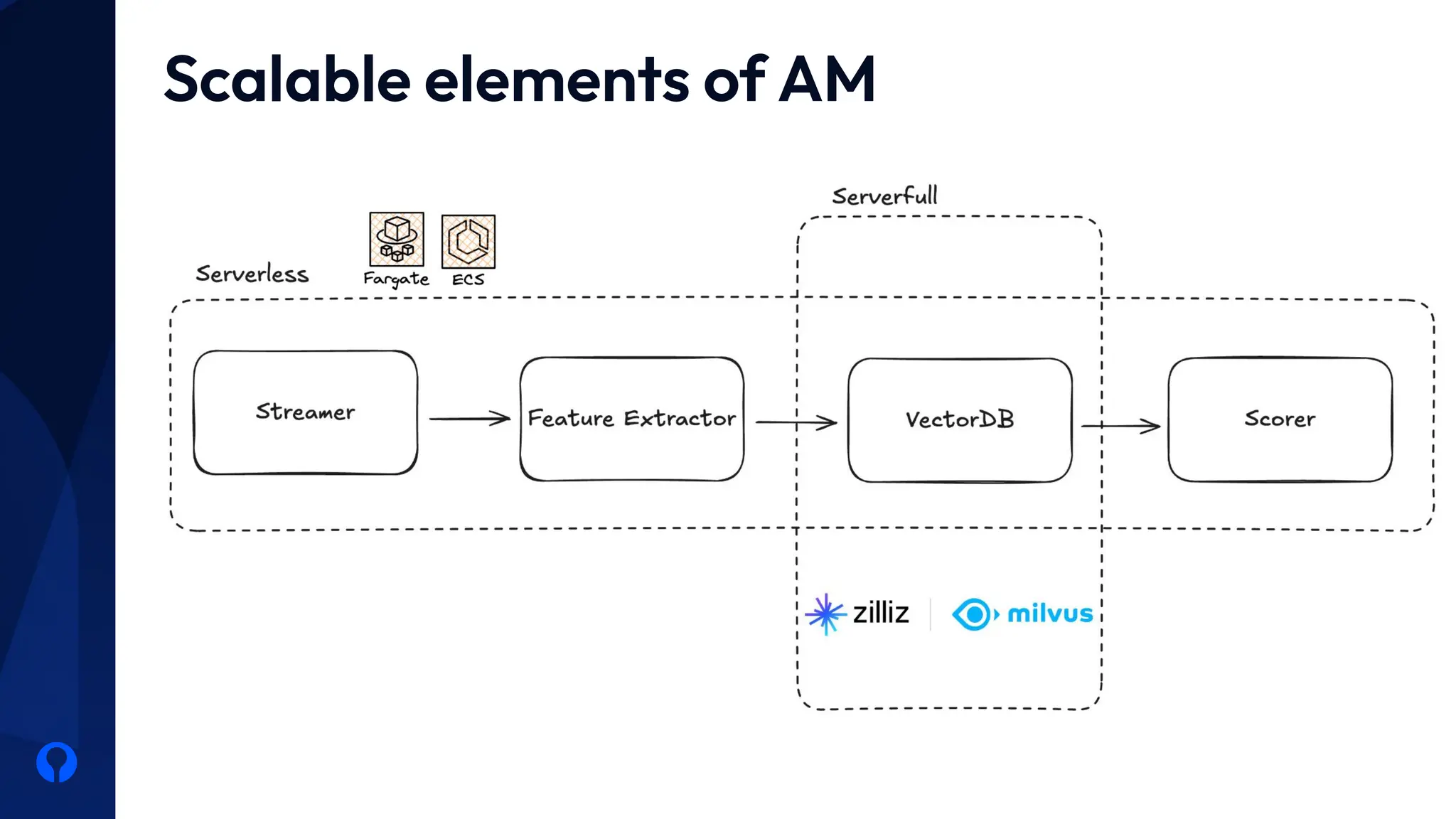
Scalable elements of AM
VectorDBs:
The 💙 of Retrieval
01
05
➜ Embeddings: meaningful representations of data that
can express similarities by their distance on an
embedding space.
➜ Text: word embeddings represent words in a way that
similar words are placed close to each other in the
embedding space, reflecting their semantic or
contextual relationships.
➜ Audio: Similarly, audio embeddings capture audio
characteristics in a way that similar sounds can be
close to each other in the embedding space.
➜ Vector DBs: A vector index with fast search abilities to
the rescue!
Vector DBs
why we need them
Find the Nearest Neighbour? Easy!
Find the Nearest Neighbour in a billion
scale problem? Not so fast :(
Compute 0.5B Euclidean Distances per
query:
1. 256 * 0.5B subtractions
2. 256 * 0.5B multiplications
3. 256 * 0.5B additions
Sum: 384B operations
Find the Approximate Nearest Neighbour? Faster!
Source:pinecone.io
IVF parameters
Source:pinecone.io
How about some compression?
Source:pinecone.io
IVFPQ Key Points
➜ IVF helps in avoiding exhaustive search the whole vector search and converts the nearest
neighbour problem in a two tiered problem.
➜ PQ helps with the compression of the data and saves space in storing and loading the
data in the vector DB.
➜ More importantly, it saves time on search and converts the demanding intrapartition
exhaustive search in a scalable table lookup.
➜ However, this comes at a price. Recall is not looking great and needs high number of
subvectors to achieve good performance.
NSW (Single Layer)
Source: Vyacheslav Efimov @ Medium
HNSW
Source: Vyacheslav Efimov @ Medium
HNSW-IVF Comparison
IVF HNSW
Algorithm Concept Clustering and bucketing Multi-layer graph navigation
Memory Usage Relatively low Relatively high
Index Build Speed Fast (only requires clustering) Slow (needs multi-layer graph construction)
Query Speed Fast, depends on nprobe Extremely fast, but with logarithmic complexity
Recall Rate
Depends on whether compression is used;
without quantization, recall can reach 95%+
Usually higher, around 98%+
Use Cases
When memory is limited, but high query
performance and recall are required
When memory is sufficient and the goal is
extremely high recall and query performance
Conclusions
01
06
➜ Designing AI services at scale can be a headache and
it is always driven by our requirements.
➜ Especially in a service with multiple models/modules
the number of options can be overwhelming.
➜ This is a blessing in disguise as it provides flexibility on
choosing and combining different setups.
➜ Tools for tracking, model versioning and
experimenting is vital for keeping this organised.
➜ All these require an orchestration layer to adapt each
use case to a specific flow that has been optimised to
work cost efficiently and satisfying the use case’s
requirements.
Conclusions
© Orfium. All rights reserved.
Kostas Eftaxias
Staff Data Scientist
Email / kostas.eftaxias@orfium.com
Linkedin / Konstantinos Eftaxias
Thank you

10 PyData Piraeus Meetup: Retrieval and Matching at Scale: from embeddings to payouts in music rights

  • 1.
    Retrieval and Matching atScale: from embeddings to payouts in music rights
  • 2.
    01. Introduction 02. Services 03.Lifecycle 04. Scale 05. VectorDBs 06. Conclusion Agenda
  • 3.
  • 4.
    Who we workwith Music Publishers Digital Service Providers Production Music Companies Record Labels Collection Societies Networks & Broadcasters Film Studios VODs & SVODs Producers (TV & film)
  • 5.
    Claiming Revenue AI servicesthat can identify music even in instances where audio has been manipulated or remixed. Catalog Management Revenue Catalog Matching at scale to help overcome ineffective handling and commonplace errors that directly impact revenue. Cuesheets AI models are utilised to eliminate manual handling of incoming documents with tabular information. How we help them?
  • 6.
    3Q 2.6M Data rowsprocessed by Orfium, 2024 Recordings matched to compositions in 2024 30k 52M Hours of video uploaded hourly to Youtube, 2024 Music recognitions in 2024 Some Numbers for Scale
  • 7.
  • 8.
  • 9.
    Metadata Based Services AutotaggingService ➜ A tagging service to categorise the audio by using its metadata. ➜ Some classes are music, audiobooks, sound effects, wellness etc. ➜ Attempts to utilise audio in a single or multimodal way benefit only specific classes. ➜ A catalog matching service that matches millions of rows vs millions of rows trying to find matches between recordings and compositions. ➜ As the process runs once a month, ephemeral OS indexes are deployed and used to generate potential matches that are evaluated by ML models. Metadata Linking Service
  • 10.
    Audio Based Services Music/NoMusic Service ➜ Simpler than Audiomatch but nevertheless helpful Service that detects segments that music is present in a track. ➜ MnM utilises a trained music detection model and its strength is its high throughput. ➜ The Core service for User Generated Content Matching process thousands of audio hours to match against our clients’ music. ➜ A multistep modular service with multiple AI models utilising a VectorDB at its core. AudioMatch Service
  • 11.
    Orchestration Layer akaCthor One layer to rule them all
  • 12.
  • 13.
    Let’s focus onAudioMatch
  • 14.
    Let’s focus onAudioMatch
  • 15.
  • 16.
    Release Checklist ➜ Basedon the changes in models/code we mix and match different tests from a range of datasets/scenarios to evaluate metrics compared to current production. ➜ We take our decision on release based on the business requirements at that point.
  • 17.
    ML Lifecycle Example 1.A novel architecture is studied or a new version of our foundation model is released. 2. We use our training module to fine tune the model based on our needs (dimensionality/focus). 3. We run a couple of benchmarks and small scale datasets for POC results in retrieval metrics. 4. If successful, we package to onnx and use the combination of optuna/ray/wandb to finetune hyperparameters. 5. If successful we push the model to DVC and using our experimentation pipeline and ClearML we start running the release checklist for synthetic and scaled datasets. 6. If the retrieval metrics are sufficient, we use the service’s environment to perform stress tests (Locust) and estimate the maximum and baseline throughput. 7. If all goes well, we merge and we have a new model in production.
  • 18.
    The three pillarsof performance
  • 19.
  • 20.
    320k audio hours wereprocessed last month 500x 1000x This is the current baseline to be able to serve our day to day needs. This is the desired peak throughput to accommodate spikes. Throughput
  • 21.
    ~1B 64-256 Vectors inVectorDB Dimensionality of the vectors 1M -10M ~250 Tracks to match against Embeddings per track Scale in VectorDB
  • 22.
  • 23.
  • 24.
    VectorDBs: The 💙 ofRetrieval 01 05
  • 25.
    ➜ Embeddings: meaningfulrepresentations of data that can express similarities by their distance on an embedding space. ➜ Text: word embeddings represent words in a way that similar words are placed close to each other in the embedding space, reflecting their semantic or contextual relationships. ➜ Audio: Similarly, audio embeddings capture audio characteristics in a way that similar sounds can be close to each other in the embedding space. ➜ Vector DBs: A vector index with fast search abilities to the rescue! Vector DBs why we need them
  • 26.
    Find the NearestNeighbour? Easy!
  • 27.
    Find the NearestNeighbour in a billion scale problem? Not so fast :( Compute 0.5B Euclidean Distances per query: 1. 256 * 0.5B subtractions 2. 256 * 0.5B multiplications 3. 256 * 0.5B additions Sum: 384B operations
  • 28.
    Find the ApproximateNearest Neighbour? Faster! Source:pinecone.io
  • 29.
  • 30.
    How about somecompression? Source:pinecone.io
  • 31.
    IVFPQ Key Points ➜IVF helps in avoiding exhaustive search the whole vector search and converts the nearest neighbour problem in a two tiered problem. ➜ PQ helps with the compression of the data and saves space in storing and loading the data in the vector DB. ➜ More importantly, it saves time on search and converts the demanding intrapartition exhaustive search in a scalable table lookup. ➜ However, this comes at a price. Recall is not looking great and needs high number of subvectors to achieve good performance.
  • 32.
    NSW (Single Layer) Source:Vyacheslav Efimov @ Medium
  • 33.
  • 34.
    HNSW-IVF Comparison IVF HNSW AlgorithmConcept Clustering and bucketing Multi-layer graph navigation Memory Usage Relatively low Relatively high Index Build Speed Fast (only requires clustering) Slow (needs multi-layer graph construction) Query Speed Fast, depends on nprobe Extremely fast, but with logarithmic complexity Recall Rate Depends on whether compression is used; without quantization, recall can reach 95%+ Usually higher, around 98%+ Use Cases When memory is limited, but high query performance and recall are required When memory is sufficient and the goal is extremely high recall and query performance
  • 35.
  • 36.
    ➜ Designing AIservices at scale can be a headache and it is always driven by our requirements. ➜ Especially in a service with multiple models/modules the number of options can be overwhelming. ➜ This is a blessing in disguise as it provides flexibility on choosing and combining different setups. ➜ Tools for tracking, model versioning and experimenting is vital for keeping this organised. ➜ All these require an orchestration layer to adapt each use case to a specific flow that has been optimised to work cost efficiently and satisfying the use case’s requirements. Conclusions
  • 37.
    © Orfium. Allrights reserved. Kostas Eftaxias Staff Data Scientist Email / kostas.eftaxias@orfium.com Linkedin / Konstantinos Eftaxias Thank you