


![,
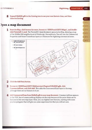
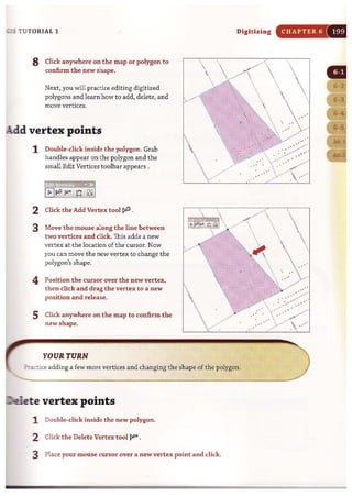
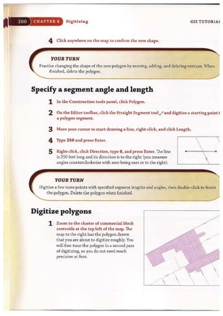
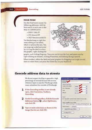
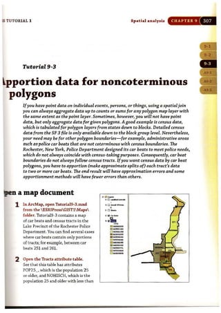
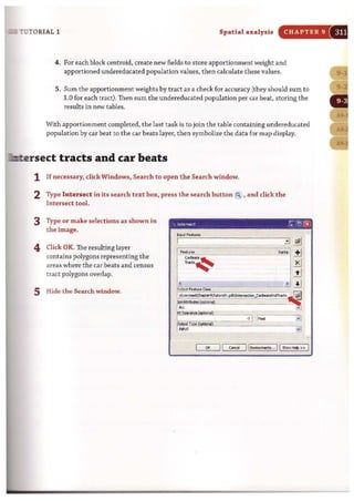
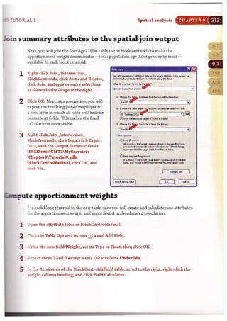
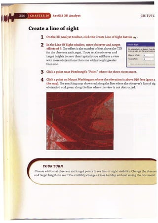
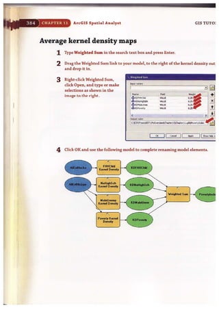
X ~I PREFACE GIS TUTORIAL 1
map address data as points through the geocoding process. Chapters 8 and 9 cover spatial
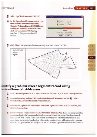
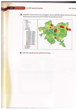
analysis using geoprocessing tools and analysis workflow models.
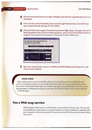
Chapters 10 and 11 provide instructions on two ArcGIS extensions. Chapter 10 introduces
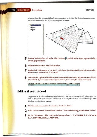
ArcGIS 3D Analyst, allowing students to create 3D scenes. conduct fly-through animations,
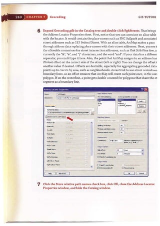
and conduct line-o(-sight studies. Finally, chapter 11 introduces ArcGIS Spatia] Analyst for
creating and analyzing raster maps, ind uding h Ulshades, density maps, site suitability
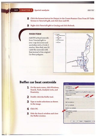
surfaces. and risk index surfaces.
Tn f",infor('!;' t he skills learned in the step -by-step exercises and to provoke critical problem-
solving skills, there are short Your Turn assignments throughout each chapter and advanced
assignments at the end of each chapter. The quickest way to increase GIS skills is to follow
up step-by-step instructions with independent work, and the assignments provide these
important learning components.
This book comes with a DVD containing exercise and assignment data and a DVD contain-
ing a trial version of ArcGIS Desktop 10, ArcEditor license. You will need to install the soft-
ware and data in order to perform the exercises and assignments in this book. (If you have
an earlier version ofArcView,ArcEditor, or Arclnfo installed, you will need to uninstall it.)
The ArcGIS Desktop 10 DVD provided with this book will work for instructors and basic-
level students in exercise labs that previously used an ArcView license of ArcGIS Desktop.
Instructions for installing the data and software that come with this book are included in
appendix D.
For teacher resources and updates related to this book, go to www.esri.coIII/ esr"ipress.](https://image.slidesharecdn.com/gistutorial1basicworkbook-130505153606-phpapp01/85/Gis-tutorial-1-basic-workbook-3-320.jpg)


![I5nJTORIAL 1 Introduction CHAPTER 1 : 7
6 Right-click COCounties in the TOC and click Remove. This action removes the map layer
from the map document but does not delete it from its storage location.
lsing relative paths
When you add a layer to a map, ArcMap stores the paths in the map document. When you
open a map, ArcMap locates the layer data it ]leeds using these stored paths. If ArcMap
cannot find the data for a layer, the layer will still appear in the ArcMap TOe, but of course
it will not appear on the map. Instead, ArcMap places a red exclamation mark (1) next to
the layer name to indicate that its path needs repair. You can view information about the
data source for a layer and repair it by clicking the Source tab in the Layers Properties
window.
Paths can be absolute or relative. An example of an absolute path is C:ESRIPressGIST1
DataUnitedStates.gdbUSCities. To share map documents saved with absolute paths,
everyone who uses the map must have exactly the same paths to map layers on his or her
computer. Instead, the relative path option is favored.
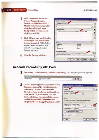
Relative paths in a map specify the location
of the layers relative to the current location
on disk of the map document (.mxd file).
Because relative paths do not contain drive
letter names, they enable the map and
its associated data to point to the same
directory structure regardless of the drive
or folder in which the map resides. Ifa
project is moved to a new drive, ArcMap
~ill still be able to find the maps and their
data by traversing the relative paths.
1 crick File, Map Document Properties.
~rotice the option is set to Store relative
pa.thnames to data sources.
.2 Click OK .
3 Save your map document.
"""",
T..,.Mte:
lMtSlYod,
lMt Pmte<J:
lMt Elq>ortod,
""d
(,ESRIPre« GlSTI1Mo!><lo.DJria1H ."",d
~.1.mxd
l-toArcGIS
Normol.mxt
1/22/2010 8:lt::t6 PM
Geo<Iot<ob....: (:Doc_ and Set!hgsl(rlston KI.riondI,AppI
F..u.-.....05t,...,~.p~to Mt~ $<M.r<O>
TlurtJnaI: ',.. " .
...:](https://image.slidesharecdn.com/gistutorial1basicworkbook-130505153606-phpapp01/85/Gis-tutorial-1-basic-workbook-15-320.jpg)

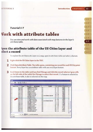
![::U AL 1 Introduction CHAPT BR 1
Iuto Hide for the Catalog window
~otice that when you opened the Catalog window, it opened in pinned-open mode, which
keeps the window open and handy for use, but covers part of your map. The Auto Hide
feature of this application window along with other application windows {such as the TOC
and Search window}keeps the windows available for immediate use, but hides them in
berween uses so that you have more room for your map.
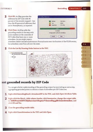
1 Click the Auto Hide button on top of the Catalog window £I..The window d oses but
leaves a Catalog button on the right side of the ArcMap windowlll.clltllbo] i.
2 Click the Catalog button. The Catalog window opens. Next, you will simulate having
completed a Catalog task by clicking the map document. The window will auto hide.
3 Click any place on the map or TOe. You can pin the window open again, which you will
do next.
4 Click the Catalog button and dick the Unpinned Auto Hide buttoniii .That pins the
Catalog window open until you dick the pin again to auto hide or dose t he window. Try
clicking the map or TOC to see that t he Catalog window remains open.
5 Close t he Catalog window.
....iii . i "_.£'~'",
YOUR TURN
!::.::e.-d.d Data or Catalog button to add COStreets, also found III ESRIPressGISTl Data
~.....es.gdb. These are street centerlines for Jefferson County, Colorado. You may have
n..:....-. seeing the streets because they occupy a small area of the map (look carefully above the
~ ::i Colorado). Later in these exercises you will learn how to zoom in for a closer look at
w...... ::eatures such as the streets.
_-_______ _ _ .."_"'_"___._.M..""'_"__.......,......,,.....,,__,~........_..-.,......~..._.;"".~,,"](https://image.slidesharecdn.com/gistutorial1basicworkbook-130505153606-phpapp01/85/Gis-tutorial-1-basic-workbook-17-320.jpg)

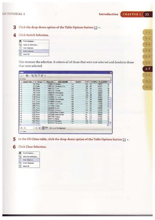
![Introduction CHAPTER 1
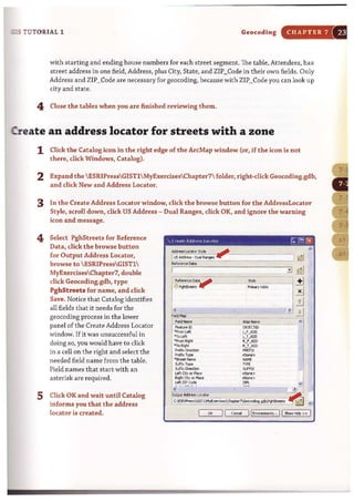
3 Drag t he usCities layer to the top of the TOC and drop it. ArcMap now draws the
US Cities last, so you can see its points again.
•::: 5!1 COStroot.
- 0 COCoosties
o
;;;: 0 US 'State,
o
•
•
• t---!:1 ~~• •i-C.~
' . J •
..•
baDge a layer's color
.,
•
•
One of the nicest capabilities of ArcGIS is how easy it is to change colors and other symbols
Ill: layers. First you will change the color fill of a layer's polygons.
S ~-3 lftyer.
E3 Ii"! USQlos
1 Click the COCounties layer's legend symbol in the TOC. The legend
sr:nbol is the rectangle below the layer name in the TOC.
•!iii Ii2I COStroots
2 Gick the Fill Color button in the Current Symbol section of the Symbol
Selector window.
3 Click the Tarragon Green tile in the Color Palette,
4 Click OK. The layer's color changes to Tarragon Green on the map.
"'No coloiu
•
[] !~:; d C O __' U ri (J8ifJr,:,
:::: m: m: nif-I CE i" c..:' If: ~ .
~ ::~~ :~~ : : :
• • • • ,,;; 8 :•• 111 • • •
:.: ~ ~ ~:.~~;-&":*~:
• .lIl U." C [] LJ lJ f' ;;; !if 1I lIE
. !l lIi m !! m~ s IlUIl . 1II
. ... .. .. m••• •
MoreCoior.".](https://image.slidesharecdn.com/gistutorial1basicworkbook-130505153606-phpapp01/85/Gis-tutorial-1-basic-workbook-19-320.jpg)


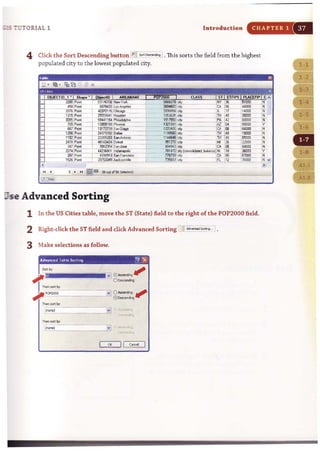
![I-::-~c' 1 Introduction CHAPTER 1
e selection symbol
:::. K";'tion to changing the color of selected features. you can change the symbol for the
~ :nap or for individual layers.
1 '='..<g'3:-click the US Cities layer in the TOC.
2 .::lic:k Properties. The resulting tabbed Layer Properties window is one that you will use
~... it allows you to modify many properties of a map layer.
3 ::x.:L the Selection tab and Symbol button.
':..::,=""",",;"""F""o,o....,_ _,.....;],;.!.!'"...lJ.<.,,"-"""']
S <.er>;Iht ....... cob ~ .. 5--... ~ I
C ....li>o 1)OI'boI . ;
I I
.J
4. :- . a new symbol and/or
.:mIc:r for point features, and
.::l:id. OK twice.
S)'nlbol ~lKlor ff}?<l
:> .:lick a d ty feat ure to see
::=enew selection symboL
.:J.e::ar the selected features.
~"""" " """-C', v
•'"
~: .
-"', 0 ....~ O Rele<encedS¥es
r ..., ..- ;.1
• • .. ,
--1
"'" ,.,." ,-,
• • •"......' -, ""- ,
• • Ii
lind S<p.Io<. 1
"'"
-".. • •TI'iarge 2
-' ......' I
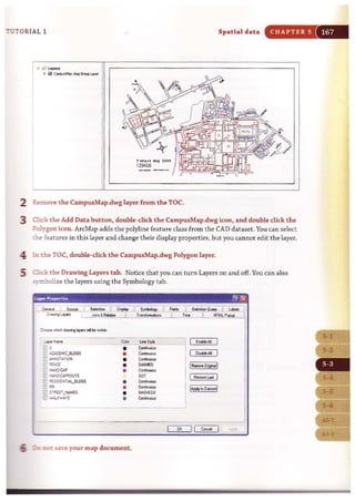
L •.-,--.-~-.
I I
~:. I
'"""-•
"",,
~
"., fiiloo -:
..,. L~__': I
I ~cI: SyIrixl",
I ,..../10... II ~
5tyW R«.."""..."
'" I ""'"](https://image.slidesharecdn.com/gistutorial1basicworkbook-130505153606-phpapp01/85/Gis-tutorial-1-basic-workbook-37-320.jpg)


![GIS TUTORIAL 1 Map design CHAPTER 2
Add a layer to the group
1 Click the Group tab in the Group Layer Properties window.
2 Click the Add button and navigate to ESRIPressGIST1DataUnitedStates.gdb.
3 Hold down the Ctrl key.
4 Click USStates and USCounties. Release the Ctrl key, then dick Add and OK.
Group Layer Properll~s !1J~
OK II Ci>f1Cd II AWl
ArcMap displays the U.S. counties with a random color.
'" i1 lay~..
S Ii!! Po!>Uatb'1 By Coorty
8 Ii!! uscOOXJties
o
~ Ii!! USstet. ,
o
'" r;;>] PopojotIon bystet.
~~,
D 5Z317'1·1993'195
D 1'193'1% . 1663715
. 4663716 · 7662029
. 7862030 ·131222%
. 131222'17 ·37'183'1'11,1
iI
I
j](https://image.slidesharecdn.com/gistutorial1basicworkbook-130505153606-phpapp01/85/Gis-tutorial-1-basic-workbook-61-320.jpg)


![;15 TUTORIAL 1 Map design CHAPTER 2
4 Click the General t ab.
5 Click the Don't show layer when zoomed radio button.
6 Type 8,000,000 in the Out beyond field and click OK. If you zoom out beyond this scale,
the layer will not be visible.
"~~r Propertle~ . . . . mIlK!
Credits: L..__ _. _ _ ---,-
5t~ Ri>"JQe
YOU ,lin >p<dy the r""'90 of ..ole. 01: ...toch this layer .. be shown:
o5how I.oyo< 01: II ..~Io. ...I/IJ,
000n~ .r- l.oyer l¥hen~: ~
0tJ; beyond: pi:~;~---- ___I~! (-.."wje);
In beyor>J: [~!0~__":"'---·:;t (m. xm....n<c.) !
_ ......~~_...._ ._.__...._.-.JOK I I c..cel I I AWl
The census tracts for Nevada disappear in the map display. ArcMap does not show the
Nevada census tract polygons when zoomed out past a scale of 1:8,000.000 as shown below
i''-'ith a scale of 1:34,453,384.
~)7;i!:.e.•~i3B4~'..C:,,;:..C.~"'.-~l:~C~O;;.c.Cc·O':J'J:JF:::-:..~:.,:.c.•,-~"'''~.'..~.-J:"c·:;J,'•.ill",c.,..~cJ",~;-:.c.co,,;-~"?.-.'".--c.:
~ s:! "wJoI;"" By Ce<lSU< Tract
= !l USstot..
Cl
-= '" l/TT,00;(.
~
D O.(n))l(J • JoJi7.00JClXl
1!!] :)(I67.t(W))J l· SJeJ.W:W
. ~3.COO')(Il· 7%1.00:wi
_:~=;-':~1- _ 1ImCDI I
- , .
:::J O.ooxm ·JH1.00xm •
• :I+<1.0000:J1- Ol O1.()"JCOJOi
• ,,01 .oooo:J! - IOOZO.ocvo'
:::::: :':=:l~'-" ='~9yC"""'t
= =~ 9y5tol:o
~ D I~ " II c " ; > ;](https://image.slidesharecdn.com/gistutorial1basicworkbook-130505153606-phpapp01/85/Gis-tutorial-1-basic-workbook-69-320.jpg)


![GIS TUTO RIAL 1 Map design CHAPTER 2
4 Continue clicking the break values above the last one changed and enter the following:
16,000,000; 8,000,000; 4,000,000; and 2,000,000. Let the last (maximum) value
remain 37,483,448.
Clau,hcal10n P?'1)(1. ,,,"
a..*-' [!i;-'---'-~~..l
dossf"~otlon Stotisto:s
Mothod, ........... .--J"
00.....' ,
""'~ £xckI<ion
,
I ~,,· I !~ .. I
C...........: [Too ': I O_Sb<I·De•.
0 __
'U ~ ! ~,
•
'til lII! l''Ib
:.m~,1mIii II I52311( 876J243 19o13311 292U390
o~ tooHks <0 dat. vo/uN
5 Click OK.
6 Click t he gray Label heading to the right
of the gray Range heading, then click
Format Labels.
7 In t he Number Format dialog box, select
Show thousands separators and click OK.
,.."~,
.......,
~ ,
-,...."
51.,.wd 0e.IeIbl:
•
!I
I
JH9JU9
lDotrlont> h o.JJ
~
5<::117'1
V_,
~-621161~
"""".......
........ 8
p::::::: l
' ""'"I,...,., ,
I ~
I
~
UI
I
~
I
""" I
--0 le11
O AVI: I =:J """'aceer.
oShow ~~• ••pllot.... - ,
E] Ptd .......'"
oShow pkn .i71
f.......~f,.·h~druTt>er;:-·
OK II c.r.:..L I](https://image.slidesharecdn.com/gistutorial1basicworkbook-130505153606-phpapp01/85/Gis-tutorial-1-basic-workbook-73-320.jpg)


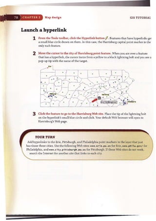
![CHAPTER 2 Map design GIS TUTORIAL ]
7 Click the Capital! symbol from the Civic symbols. Click OK.
8 Click the General tab and change the layer name to State Capital.
9 Click OK. The resultant map shows medium-sized cities, county seats, and
the state capital, Harrisburg.
YOUR TURN
Copitoi 1
CIvil:
Add the PACities layer once more and create a definition query that displays Pennsylvanl'i'~
three largest cities: Erie, Philadelphia, and Pittsburgh. Rename the layer "Major Cities",and sho":
the three cities with a symbol that makes them stand out on the map, Hint: One sol~tiori,is tb
use the query "NAME" '" 'Erie' OR "NAME" = 'Philadelphia' OR "NAME"=" Pittsbu.rgh', See if you
can create halo labels for this layer and the State Capital layer.](https://image.slidesharecdn.com/gistutorial1basicworkbook-130505153606-phpapp01/85/Gis-tutorial-1-basic-workbook-84-320.jpg)


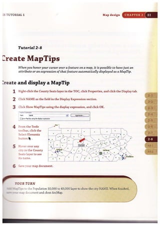


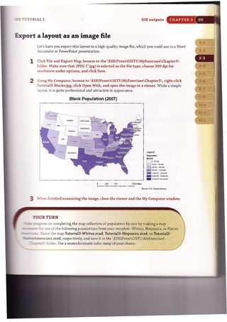
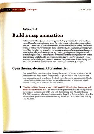
![:;:s TUTORIAL 1 GIS outputs CHAPTER 3
2 In the ArcMap - Getting Started window, dick Browse for more. Browse to the drive where
you inst alled ESRIPressGIST1Maps' and double-click TutoriaI3-1.mxd. Tutoria13-1.mxd
opens in ArcMap showing a map of the United States with state capitals displayed. Notice that
the map document has visible scale ranges set, indicated by the grayed-out check boxes in the
table of contents (TOC) for layers not visible at the starting scale.
;;; & l · r·...
",Q ~ .,.Cout.,
'" Q 0;"
,-~
• ". 10,000
0 10,"'" ·so.ooo
a so,oo, ·100,000
8'","00' .500,000
500,00' · 1,000,000
0 ,,000.001on;! 0;._
1;< Cl ,.",,8oood_
C]
.0_""'-D o-<oo,OOJ
D <oo.001· '00.000
111-000,001. "",000
. 0CI.l,001. 1.600.000
. uoo.Cl:n · J,>OO,OOO
. ' .>00,001""'"""",
- 8 P<l«Jotm.,.,..,.
"" "",..,.Cool""
*; 8 ""'..
...-D e· 2,ooo,ooo
0 2,OOJ,00, ·',OOJ,OOO
111<,000,00' · O.OOJ,OOO
• • •00J.00, • 16.00J,000
• 16,00J,00' . 3<.000.000
. ).1.000.00 ' '''",,,,,,,,
3 Click File and Save As, browse to the ESRIPressGISTlMyExercisesChapter 3 folder,
and click Save.
4 Click the Hyperlink tool fIon the Tools toolbar and click the st ate capital of your choice
all features that have hyperlinks get blue dots). If the Tools toolbar is not open, click
Customize, Toolbars, Tools on the main menu. Your Web browser opens to that state's
=-government Web page. Here you might find information about recreation in the state or
S"".2.te subsidies or tax relief for opening new retail sites. Close the browser.](https://image.slidesharecdn.com/gistutorial1basicworkbook-130505153606-phpapp01/85/Gis-tutorial-1-basic-workbook-96-320.jpg)
![GIS outputs
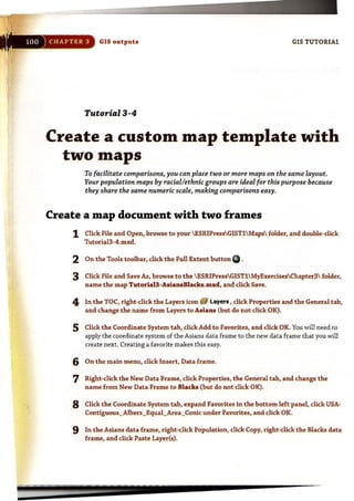
6 Use the Zoom In button
~ and Pan button ~ to
make the map larger and
centered.
7 Select 100% on the Layout
toolbar and use scroll bars
to view the legend, scale
bar, and text.
8 Click the Zoom Whole Page
button E;] on the Layout
toolbar.
9 click File and Save As, and
save your map as
ESRIPressGISTl
MyExercisesChapter3Tutoria13-2a.mxd.
YOUR TURN
GIS TUTORIAL J
Save TutoriaI3-2a.mxd as ESRIPress GISTlMyExerdsesChapter3Tutoria13-2b.mxd. Click )
the Change Layout button ~ and use a layout template of your choiCe. Change the title of the
layout toAsianpOPul~t~onbY..~tatein2007 , . . _, __,~
Save a layer file
The set of layouts that you wiU produce below are for wmparing populations by race or
ethnicity for states. Next, as a preliminary step, you will create a layer file that saves the
symbology of a map layer for reuse. To facilitate comparisons of populations by race on
separate maps, it is desirable to use the same numeric scale for all maps. So as part of the
work, you will save a layer file that allows easy reuse of a numeric scale.
1 Click File and Open, browse to your ESRIPressGISTlMaps folder and double-dick
TutoriaI3-2.mxd (the same map document you used in the previous exercise).
2 Click File and SaveAs, and save your map document as ESRIPressGISTlMyE.:ar:ercises
Chapter3TutoriaI3-Asians.mxd,](https://image.slidesharecdn.com/gistutorial1basicworkbook-130505153606-phpapp01/85/Gis-tutorial-1-basic-workbook-99-320.jpg)

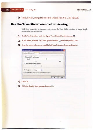
![IS TUTORIAL 1 GIS outputs CHAPTER 3
:reate and use guidelines in the layout view
In the next steps, you will use vertical and horizontal rulers to create guidelines.
1 Click at 8.5 inches on the top horizontal ruler to create a vertical blue guide at that
location. If you place your guide at the wrong location, right-click its arrow on the ruler,
click Clear Guide, and start over.
2 Do the same at 7 inches on the left vertical ruler.
3 Click the map to select it (dashed outlines and grab handles appear), right-click the
map and click Properties, then click the Size and Position tab.
4 Click the Preserve Aspect Ratio check box, type 7.S in the Size Width field, press the Tab
key, and click OK.
5 Drag the map so that its upper right corner is at the intersection of the two guides, and
release. The map snaps precisely to the intersection of the guides when you release. The
objective of the next step is to fill the map element rectangle with the map as large as possible.
6 Use the Zoom In button ~ on the Tools toolbar to drag a rectangle around just the
physical map itself to increase the size of the map within its map element rectangle.
If you need to start over, click the Full Extent button Q) .
... .. .. - .....- .....- .... -.- ..- -----.-- ---- -.-...--.......-.-. ...... ..0
0.-- --,- -- ---.------ -.---- - --- ---- --- --- -- -----.------- --- -- -- .---.{]](https://image.slidesharecdn.com/gistutorial1basicworkbook-130505153606-phpapp01/85/Gis-tutorial-1-basic-workbook-102-320.jpg)


![~ TU T O RIAL 1
._,[] "iQT,
Iii 0 CAD Col. C<TI;ext
N.ru, codo
.~,
GIS outputs
2 Click File and Save As, browse to ESRIPressGIST1MyExercisesChapter3,
and click Save.
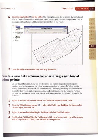
Set time properties of a layer
CHAPTER 3
1 Right-click CAD Calls in the TOC, click Properties and the Time tab, and type or make
selections as follows. CALLDATE has dates such as 7/1/2009. The Time Step Interval is
~e unit of time for measurement, here 1 day.
I I](https://image.slidesharecdn.com/gistutorial1basicworkbook-130505153606-phpapp01/85/Gis-tutorial-1-basic-workbook-122-320.jpg)


![Part
Working with spatial data
, , c , f
• ".811'5 geographic
n syste ms g e ogr'ap hic
.~" ', ' phic
nfo'rr.':ILi n syste ms
jnfol~mation systems
infor mation systems
geograph c
geor~raphic
9~ographic
gEographic
geographic
geogr' aphi c
or' matio o
c information
c inforM.;tion
c "r, o'"mati "
systems
terns
raph
;:, geograp
~yste ms geograph c
systems geograp tlic
systems geog r aphic
syste$s geographic
s)' S ..: ,-, D 5 98- 09 ra oh i C
1·.. Q::, t~dpn
eograph
jPogrr]oh
1 ' :, ," , <:'tio'" '::l.G'S' ['Qq,-
File geodatabases
_:::.-~-.o": can directly use or import most GIS file formats in common use for
1-'25:X" es~ing and display. The recommended native file format for use in
""";:".~.... !3 the file geodatabase that stores map layers, data tables, and other
- e-::pes in a system folder that has the suffix extension .gdb in its name.
~ +.:-z;ter you will learn about working with file geodatabases.
n f ,
in ( I
in f I
i n f,
in f I
in f I](https://image.slidesharecdn.com/gistutorial1basicworkbook-130505153606-phpapp01/85/Gis-tutorial-1-basic-workbook-131-320.jpg)

![,
1
i
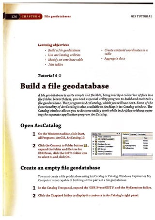
File geodatabases GIS TUTORIAL]
Tutorial 4-2
Use ArcCatalog utilities
Now that you've created a file geodatabase, you can start usingArcCatalog's
utilities. First are the preview utilities, which give you a good overview ofa feature
layer or table.
Preview layers
1 Click MaricopaCountyFiles.gdb to expose
its contents in the right panel.
2 In theright panel, click tgr04013ccdOO and
click the Preview tab. ArcCatalog previews
the tgr04013ccdOO map layer's geography.
3 At the bottom of the Preview tab, select
Table as the Preview. ArcCatalog
previews the tgr04013ccdOO map layer's
attribute table.
~,N.~.~".__.._:::Ek,['>r.?..;::~....~"~.~"
1!1ik~ Flo G.od.tobase Tobie
(Il tgr04013ccdOO FJe GeoMt_ Feot",e a-
[litgr04013O:rtOO RIo Geod.otobase foot",. a-](https://image.slidesharecdn.com/gistutorial1basicworkbook-130505153606-phpapp01/85/Gis-tutorial-1-basic-workbook-134-320.jpg)

![,
132 ) CHAP TER 4 File geodatab ases GIS TUTORIAL
Modify a primary key
It is often necessary to join two tables to make a single table. For example, there are
hundreds: of census variables, so it is impractical to have all needed census variables
for tracts stored in the tract polygon table. Instead, you select the variables you wish,
download a corresponding table from the Census Bureau Web site, and join the table to thE
tract polygon table.
For tables to join, they must share unique identifiers or keys. The STFID column of the
Tracts table and the GEO_ID column of the CensusTractData table are the corresponding
unique identifiers for these tables. These attributes would match, except that GEO_ID has
the extra characters "14000U5" at the beginning of each value. Next, you will use a string
function, Mid([GEO_ID], 8,11), that extracts an ll-character string from GEO_ID startin~
at position 8 and creates a new column in Attributes of CensusTractData to match 5TFID 0
Attributes of Tracts.
1 Right-click Tracts in the TOC and click Open Attribute Table. Note that STFID in this
table has values such as 04013010100.
2 Close the Tracts table, right-click CensusTractData in the TOC, and click Open.
GEO_ID in this table has values such as 14000U504013010100, with the extra seven
beginning characters.
3 In the CensusTractData table, click the drop-down arrow of the Table Options button
[;3 ... and click Add Field.
4 In the Add Field dialog box, type STPID in the Name field, change the Type to Text and
Length to 11, and click OK.
5 Scroll to the right in the CensusTractData table, right-click the STFID column heading,
and click Field Calculator.
6 In the Field Calculator dialog box, change the Type from Number to String; double-did
the MidO function; and in the STFID", box, edit the MidO function to Mid([GEO_ID],
8,11) and click OK. That cakuJates values for STFID in this table such as 04013010100.](https://image.slidesharecdn.com/gistutorial1basicworkbook-130505153606-phpapp01/85/Gis-tutorial-1-basic-workbook-138-320.jpg)

![',-,,
if
j
CHAPTER 4 File geodatabases GIS TUTORIAL ]
Tutorial 4-4
Join tables
Often you will need to display data on your map that is not directly stored with a
map layer. For example, you might obtain data from other departments in your
organization, purchase commercially available data, or download data from the
Internet. Ifthis data is stored in a table such as an Excel or comma-separated-value
table and has geocodes such as census tract numbers matchingyour tract map layer
you can import it into a file geodatabase andjoin it to yourgeographic features for
display on your map. Next, you willjoin the CensusTractData table to the polygon
Tracts feature class. The same steps work ifyour map layer is a shapefile or map
layer in another format supported by ArcMap.
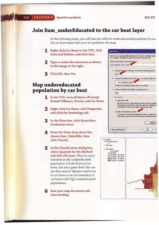
1 In the ArcMap table of contents, right-
click the Tracts layer, click Joins and
Relates, then click Join.
2 Make the selections shown in the
graphic on the right.
3 Click OK, Yes. 2. c~. tho tobIe to r.-:~ layer, or load the toble from dsk:
IIiiiI ConsusTractDl tl r - ::1 ~
oShoV.,tho ~h.t" tobIos <:i layer. In tho k t
..Join Optbns
@Keep ol records
AI record> n tho.tl'lIOt tabla Irl .hown n tt"la ,"SI.bIgtabll ,
Unmltched ..cord. .. cortaIn ..... "".for 01 fields ~
Ippended I"t,,-ha target tabla from'tho "*'tllble,
oKeep only matchinq rocordo
11 I record n th.:tl'lIOt tabla ilo.sn hove • matCh n tho jOin
tobie,·tiW recco"~ ,,~ FrOOt the resi.t~ i..1IOt table,
IIIboo,t ~ Date I or I ! CS'J«I](https://image.slidesharecdn.com/gistutorial1basicworkbook-130505153606-phpapp01/85/Gis-tutorial-1-basic-workbook-140-320.jpg)


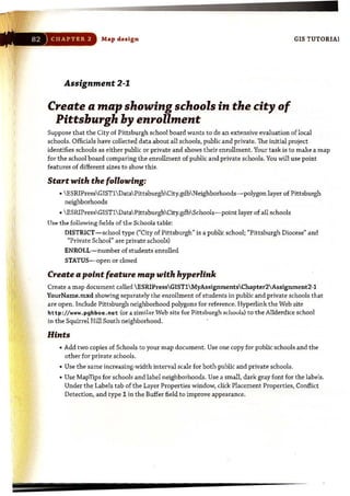
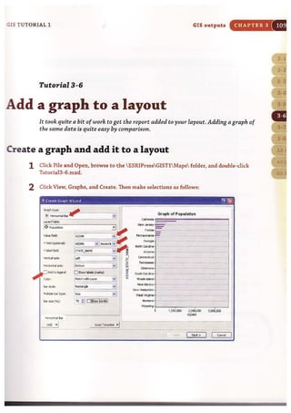
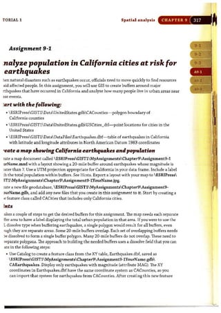
![::r:-.:::sJ.AL 1 Pile geodataballCUl CHAPTER 4
h-::~holize the choropleth map
-,',!:h counts of eating and drinking places now joined to the car beats polygon layer, you
.orre ready to create a car beat choropleth map. The resulting map will provide a good
=.eans for scanning the entire city for areas with high concentrations of crime-prone
estGblishments.
1 :light-click Car Beats in t he table of contents. Click Properties, the Labels tab, and the
::....a.bel Features in this layer check box.
2 Cck the General tab and change the Layer Name to Number of Eating and Drinking
Plac.es.
3 ::ick the Symbology tab, Quantities, and Graduated colors.
-4 ;--.mge the Value field to Count_BEAT, choose a monochromatic color ramp, and click
::.assify.
5 1:: ±e Classification dialog box, choose 7 classes, set the Method drop-down list to
~t:ile, and dick OK twice.
-
7:::rn off al11ayers except Number of Eating and Drinking Places.
..,.,.
- = ~"o<
•- = ,~.,
- .i:: ....,..,.. 01 Eot..... ..-.J Or~ fl"a<e.
CoI.n:..&AT
c ,· ]
1iJ!· 11
• L1 - 16
. 1' · ~
. 17 ·38
"roUI map document and exit ArcMap.](https://image.slidesharecdn.com/gistutorial1basicworkbook-130505153606-phpapp01/85/Gis-tutorial-1-basic-workbook-151-320.jpg)


![I
I)
i
,~
It
I
154 CHAPTER 5 Sp atial d a t a GIS TUTORlt
Tutorial 5-2
Work with map projections
There are two types ofcoordinate systems-geographic and projected. Geograpf
coordinate systems use latitude and longitude coordinates for locations on the s
face ofa sphere while projected coordinate systems use a mathematical conversi
to transform latitude and longitude coordinates to a flat surface.
Set world projections
1
Because the earth is nearly spherical and maps are fiat, GIS applications require that a
mathematical formulation be applied to the earth to represent it on a flat surface. This i
called a map projection, and it causes distortions in some combination of distance, area
shape, or direction. ArcMap has more than 100 projections from which you may choose
Typically, though, only a few projections are suitable for your data.
In ArcMap, open TutorialS-2.mxd from the ESRIPressGISTlMaps folder.
., ill' ~
Ei O!I C<U'Itry [.
o 'I0._r:;:] "
2 Place your cursor over the westernmost point ofAfrica and read the coordinates on
the bottom of the ArcMap window (approximately -16.6,21.6 decimal degrees). The
map and data frame are in geographic coordinates, decimal degrees, which are angles oj
rotation of earth's radius from the prime meridian on the equator. These coordinates al](https://image.slidesharecdn.com/gistutorial1basicworkbook-130505153606-phpapp01/85/Gis-tutorial-1-basic-workbook-160-320.jpg)

![CHAPTER 5 Spatial data GIS TUTOR1
YOUR TURN
Repeat the four steps of the previous exercise, but this time select the Hammer~Aitoff
projection in the third step. This projection is nearly the opposite of the Mercator. The
Hammer-Aitoff is good for use on a world map, being an equal-area projection ttiat preserves
area. However, it distorts direction and distance. Repeat the steps again, this time choosing the
Robinson projection. This projection minimizes distortions of many kinds, striking a balance
between conformal and equal-area projections. Do not save changes to the map document.
:: ~~ Lo,."
~ Ii!l c",-"",
o
.. Ii!] Ocoon
o](https://image.slidesharecdn.com/gistutorial1basicworkbook-130505153606-phpapp01/85/Gis-tutorial-1-basic-workbook-162-320.jpg)

![Spatial data
YOUR TURN
Experiment by applying a few other projections to the U::5:,...:6:,
Equidistant. As long as you stay in the
the projections look similar. The conclusion is that the
need to project, the less distortion. There
but much less so than for the entire world. By the
Allegheny County, practically no distortion is
your map document.
State plane coordinate system
GIS TUTOI
The state plane coordinate system is a series of projections. It divides the SOU.S. state!
Puerto Rico, and the U.S. Virgin Islands into more than 124 numbered sections referrE
to as zones, each with its own finely tuned projection. Used mostly by local governrner:
agencies such as counties, municipalities, and cities, the state plane coordinate system
for large-scale mapping in the United States. The U.S. Coast and Geodetic Survey devel
it in the 1930s to provide a common reference system for surveyors and rnapmakers. T
first step in using a state plane projection is to look up the correct zone for your area.
1 Start your Web browser, go t o www.ngs.noaa .gov/TOOLS/spc.shtr.l , and click the Fi
Zone link.
State Plane Coordinates
The s.... "'-C"",&o.I.. ')"SlCm Pf",ideJ~..
on I fto!.,,;ct b" . ..~ compl>tllrion "'hi< """'''"''''
• d&rm« b<n>'fflI'~ ODd p:io! WIoa<o <:I:
_ ~iII ]0.000«"-".
The s.... PloD< C"",diooI. 0:<,..... <ioidr< II>< u.s.ioIo
• Iuo<Rd or """'. 41..nct !rid...t.." (Z_.).
00Il0l''';' ~&om_ Z_,,1iIbtbolill-.-.
In )"" "".~ to rn", Z<J<>O ~" ... Good<-ti, Po",",,,,.
The IIIiiIios ill Ibi:s f*1<>a< ".O"Iid< IlIOdIods for C<l<I''OI"Iio,
b.I'"e'" Gfodetic Positions NId sw.. PI_ C_-...or for foIdiq III Sl'C Z-.
For ""'"' ~ ob«IIlbt ShI. PIaD< C..,..dNI. S)"<t<1II COIltOct
Tbt Na-J G...wc SIIr'oyldormoDooo Senft< Br...rn
pboao: 00]) 1 !).) :4 ~; h.,~JO ! ) i 13·41"72 [:'I!<'<I.•Fri.. 7:00 • .In. • ~:30 p.m. EST]
"'"](https://image.slidesharecdn.com/gistutorial1basicworkbook-130505153606-phpapp01/85/Gis-tutorial-1-basic-workbook-164-320.jpg)


![I
Spatial data GIS TUTORIJ
Tutorial 5-3
Learn about vector data formats
This tutorial reviews several file formats commonly found for vector spatial data
other than the file geodatabase covered in chapter 4. Included are ESRI shapefile
and coverages as well as computer aided design (CAD) files, XYevent files, and
other tabular data formats.
Examine a shapefile
Many spatial data suppliers use the shapefile data format for vector map layers because
it is so simple. Shapefiles appeared about t he same time that personal computers became
popular. Ashapefile consists of at least three files: a SHP file, DBF file, and a SHXfile.
Each of these files uses the shape61e's name but with the different file types. The SHP file
stores the geometry of the features, the DBF file stores the attribute table, and the SHX
file stores an index of the spatial geometry for quick processing. Next, you wiJ] examine
AlleghenyCountyTracts.shp in more detail.
1 Examine AlleghenyCountyTracts.shp in Catalog. It appears
as an entry in one line with an icon representing a polygon map
layer. ArcCatalog treats the several 61es as a unit and provides
utilities such as renaming the shapefile in one location. In fact,
as you will see next, there are several files that make up the
shapefile layer.
2 Open a My Computer window and navigate to ESRIPressGIST1
Data Datafiles . Now you can see that there are seven files for the
shapefile, including the projection (.prj) file that you created above
when you added a spatial reference for the layer's coordinate system.
3 Close the My Computer window.
8 E:I[)at~
!I1S22:2.1;xt
i!l2lXllsfIC<ll.lllty.ts~
Iii 2Imsfl'at....
IJIi ~Tr~
[:;:) .t.uto~~.st](https://image.slidesharecdn.com/gistutorial1basicworkbook-130505153606-phpapp01/85/Gis-tutorial-1-basic-workbook-170-320.jpg)

![,[' j,
Spatial data GIS TUTORIA
Convert a coverage to a shapefile
If you need to edit the attribute tables or geometry of a coverage, you must export it firs
the shapefile or file geodatabase format in ArcMap.
1 In the TOe, right-click the Building Polygon layer, click Data, and click Export Data.
2 Browse to ESRIPressGIST1MyExercisesChapterS and save the output sbapefile <
Building.shp.
3 Click OK, then click Yes to add the exported data to the map as a layer. Now you caul
edit the polygons in Building.shp and add the missing sp~tial reference for the layer. YOI
will learn about editing shapefiles in chapter 6.
4 Do not save your map document.
CAD files
Many organizations have CAD (computer-aided design) files, drawings that you can disl
in ArcMap in their native format. ArcMap can add CAD files in one of
two CAD formats: as native AutoCAD (.dwg) or as Drawing Exchange
Files (.dxf) that most CAD software can create. When viewed in
Catalog, a CAD dataset appears with a light blue icon. An AutoCAD
file is much like a coverage in that it has different kinds of vector
features in the same file. You can see CampusMap.dwg in ArcCatalog
in the image on the right.
Add a CAD file as a layer for display
lil BiI QlUClmpJf
'Oil ill CarnplJsMap.,
00 .......
lliJ~
e;::] PoIrt
ill _
S_
1 In a new blank map, click the Add Data button, browse to ESRIPressGISTlData
CMUCampus, dick the CampusMap.dwg icon, and Add. The following map of the
Carnegie Mellon University campus appears in ArcMap. It contains many feature types,
including lines, polygons, and text. This map is for display only.](https://image.slidesharecdn.com/gistutorial1basicworkbook-130505153606-phpapp01/85/Gis-tutorial-1-basic-workbook-172-320.jpg)


![17H CHAPTER 5 Spatial data GIS TUTORl
Tables
here: !lIil ' Q~WQ"'~ Cffiltr , Gtigr'i'hv , T. bln • ;;..~U~.
CeMu• •COO S~~'Y 'II! ) (Sf ~) . S.""'!! Oi l•. G c wnlO'~ C~nttt
• Chooile a table u lection method
• Select one or more tables and click 'Add', c,.- ----.
~
27. Pl.!ee. d 'QIk f~Wod-.en: I &. Yi!8I1"Pllce-~vel ..--. - - - - -
P28, Piace of '1011< lor 'lor1<~r1 16· Ye.~ ·,M S,I../PMS..t.. Le,·ej
P2~ Place cd 'N:.II<lor Werker116. Yeaft,M"1Or'Gd Civisi,., Level lor12St.tt. leT ME ~IA. MI IAII flH IJ.I IIY PA. RI VT w n
!Pl!. T~eI Trne I~ WOII<lO<" "",'od-".et"t 16-· Years
~
n Tr~'eI Tone te Work l'y If.e.llll IJ T~Qn ~ WCrI< IorWcrl<ers I!- YNB WIll) Cid llot '/"" & Home
p ~ ~~O$e l,11'1!1 Trne to VlWt. .... Mn.t~) by l.a·,111 T.".. by ~~ IJ Trans I~ Wor(MI 16· "e.m
P34,Trne ~a"~ 1+:roe1Q'Plo Wor.:. forWori<m j6- Yela
P35, ;:;'vlte Vel'ielt Oeeupar)C)' for WQlir.~ 1£. YUft
P)Ue:. by$ellool ~t ~J,~ of SdOOl by ])111 of_Sc!l~~t~~CJO· ~Y'"""._ ___
j Remove I
I Ne:><t .. I
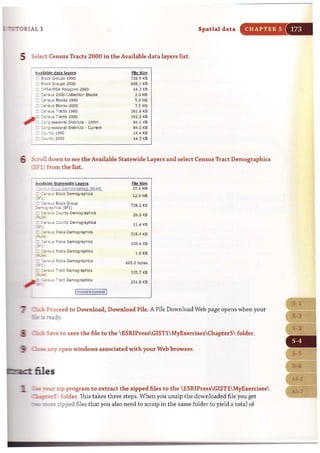
9 Click Next, Start Download. Note: This may take several minutes to download.
10 Save the resulting zippedfile to ESRIPressGIST1 MyExercisesChapterS, then extract
zipped file to the same folder, resulting in the text file dc_dec_2000_sf3_u_datal.txt.
YOUR TURN
DownlO<ld <l few SF1 cens us variables fo r Illinois census LlaLb.
" ' -_ _ _ _• _ _ _ _..m .... ...._ _..._ _......... " _. • _ _ _~ ..........._ ...............
Import text data into Microsoft Excel
The census data that you downloaded in the previous exercise as a text table needs some
cleaning up using software such as Microsoft Excel before using in your GIS. First, you
need to import the text table into Excel.
1 Open Microsoft Excel on your computer, click t he Office button @ , clickOpen, sele(
All Files (t.*) for Files of type, browse to ESRIPressGIST1 MyExercisesChapterS,
and double·click dc dec2000_sf3_u_data1.txt.
2 In the Text Import Wizard, click t he Delimited Option button, click Next, clear the 1
check box, dick Other, type the "1" character (above the Enter key) in the text box tc
t he right of the Other check box.](https://image.slidesharecdn.com/gistutorial1basicworkbook-130505153606-phpapp01/85/Gis-tutorial-1-basic-workbook-184-320.jpg)


![Jl5 TUTORIAL 1 Spatial data CHAPTER 5
Create an interactil1e GIS
Create a new map document called ESRIPressGIST1 MyAssignmentsChapterS Assignment5-
ffourName.mxd. Use scales to display detailed layers when zoomed in to 1:100,000 scale. At that
g:aje, display labels for voting districts, schools, and streets. This provides a tool for analyzing
!?fXential voting places, voting district by voting district.
Look up the state piane zone for Maricopa County and use it for your map document's data frame.
.;c'rl spatial reference data for the ESRI shapefiles: GCS_North_American_1983 (NAD 1983.prj).
"'!::en you add the x,y data, eiit the Coordinate System of Input Coordinates to use the correct
G::ae plane coordin:lte!: of Maricopa County Arizona. Add a field to block census data; Voters =
;?OP2000] - IAGE_UNDERS] - IAGE_S_17].
E-crvery small-grain spatial data, such as provided by census blocks, a good approach is to use
.s:r::aU. square point markers of the same size and with a monochromatic color ramp. Symbolize
..:Iibcks using graduated symbols for the Voters attribute and use a "trick" to make all symbols the
~ size. Use size from 4 to 4 to get same size and then double-click each symbol to change coior
.iJr the monochromatic ramp. Set the background color to No Color. The benefit of the "trick" is that
.&rl.hp uses point markers instead of choropleth maps for the blocks.
~e an ll-by-8.S-inch landscape layout with map, legend, and title. Zoom in to a populated
~of your map document with a map scale of 1:24,000. Export the layout as ESRIPressGIST1
~entsChapter5Assignment5-1YourName.jpg. Create a Word document, saved as
!SlIPressGIST1 MyAssignmentsChapterS Assignment5-1YourName.doc, that has a title,
wm:r :ld.me, your map layout image, and a paragraph suggesting schools to be used as polling places
_ cC:se:rved voting districts.
WHAT TO TURN IN
If your work is to be graded, turn in the following files:
file geodatabase: ESRIPressGIST1MyAssignmentsChapterS
AssignmentS-1YourName.gdb
ArcMap document: ESRIPressGIST1MyAssignmentsChapterS
.!.ms-runentS-1YourName.mxd
Itan:I document: ESRIPressGIST1MyAssignmentsChapterS
~entS -1YourName.doc
:l::r.age file: ESRIPressGISTlMyAssignmentsChapterS
~-nm.entS-1YourName.jpg
Jfi::::structed to do so, instead of the above individual files, turn in a compressed file,
AssignmentS-1YourName.zip, with all files included. Do not include path information
~mpressed file.](https://image.slidesharecdn.com/gistutorial1basicworkbook-130505153606-phpapp01/85/Gis-tutorial-1-basic-workbook-195-320.jpg)


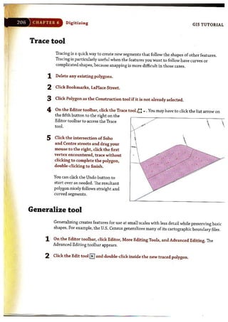
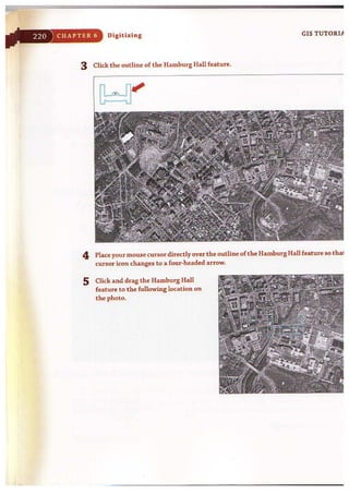
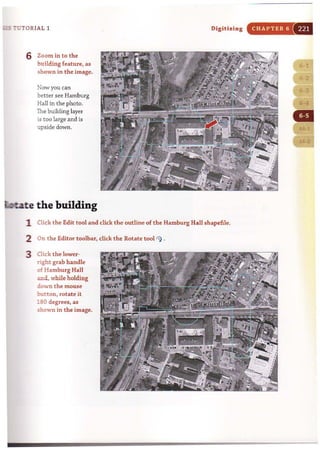
![CHAPTER 6 Digitizing
3 Click the Straight Segment tool ,/
and draw another new polygon feature
as shown in the image, snapping to
intersections.
4 Click the Edit tool G _
5 Double-click the new polygon. Grab
handles, small squares, appear on the
polygon at its vertex locations_Next, you
will see that you can edit the shape of a
feature by moving a vertex.
6 Position the cursor overone ofthe vertices.
7 Click and drag t he vertex somewhere
nearby and release_ The polygon's shape
changes correspondingly.
GIS TUTOR]](https://image.slidesharecdn.com/gistutorial1basicworkbook-130505153606-phpapp01/85/Gis-tutorial-1-basic-workbook-203-320.jpg)


![:i;. .
i'
7
Digitizing
GIS TUTOR]
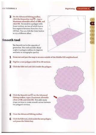
Prepare area for digitizing and start editing
1 Zoom to the western half of the Middle Hill neighborhood as shown below.
..,.
"
" :,..
"0: ••'
..: ..,.
2 On the Editor toolbar, click Editor, Start Editing.
3 Click the EvacRoute layer and OK.
4 Click EvacRoute in the Create Features panel.
Digitize by snapping to features
. :. ::'
'.;..;...- ,"
You will snap digitized lines to features to make sure that line segments connect where the
should. Make sure that Endpoint snap is on so you snap to the endpoint of the street segm!
1 Click the Straight Segment tool ./ .](https://image.slidesharecdn.com/gistutorial1basicworkbook-130505153606-phpapp01/85/Gis-tutorial-1-basic-workbook-219-320.jpg)


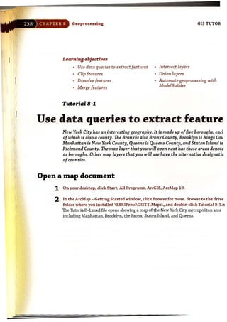


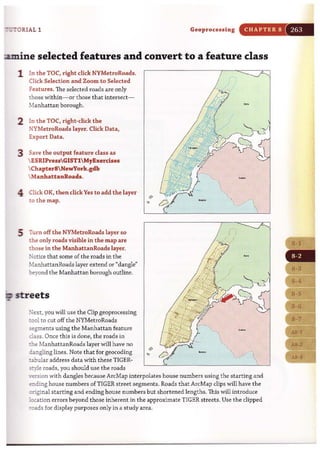
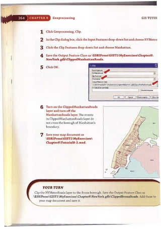


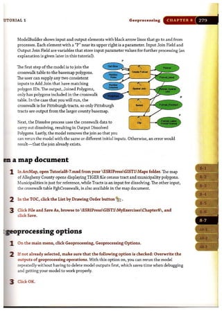

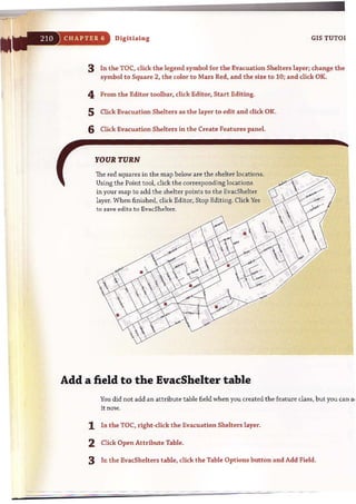
![CHAPTER 8 Geoprocessing GIS TUTOI
Dissolve tracts
1 Type dissolve in the search text box and click
the Search button ®. "'""...
2 Drag the Dissolve tool and drop it below the
Join process in your model.
3 Click the Connect button ~ on the model window's Standard toolbar, click Tracts
output from the Add Join process in the model, click the Dissolve process, and cli,
Input Featuc~t; in the resulting context menu.
4 Click the model's Select button lit .
5 Double-click the Dissolve process
in your model and make selections
using the drop-down list in each
remaining field as shown in the
image at the right (but do not click
OK).
6 Select Tracts. POP2000 in the
Statistics Field(s) and ignore the
resulting warning.
7 Click in the Statistics Type cell to
the right of Tracts.POP2000, click
the resulting drop-down arrow, and
select SUM.
8 Repeat steps 6 and 7 for two
additional attributes, Tracts.WHITE
and Tracts.BLACK, using SUM for
both. Click OK.
9 Right-click the Neighborhoods output
, () .."Ive
~':i'- ::J [
~f"".o.s. .....
! GJ5TI~a..t~.PNoVobal.....e "
~.h!!l9.!optiona!l
o T,ectf.OIII9D:. OCC
o T,oru.RfNTtR_OCC
o T,*It.5QMi
o T'ectf.~J,orIoth
o T,.KlS."-.......
O~OIO
O ~$TfIO .~
0 ~HOOO r-
i-
____ ~.... .~ ,",.1 -
El Ct.~. ",......11.~ur" [aptioM]
Iii5.;.•.
01( II c.w.:. )I A>W II Show ~
of the Dissolve process, click Add To Display, and save your model.
10 Right-dick the Dissolve process, dick Run, and close the resulting window when tJ
model has finished running.
Note: If several of your model processes and outputs lose their color fill, meaning that
input is missing, double-click the Add Join process and add Tracts as the Layer Name c
Table View. Then delete the original input that will now be disconnected.](https://image.slidesharecdn.com/gistutorial1basicworkbook-130505153606-phpapp01/85/Gis-tutorial-1-basic-workbook-287-320.jpg)


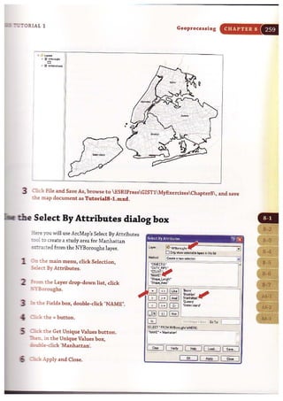
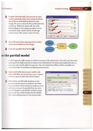
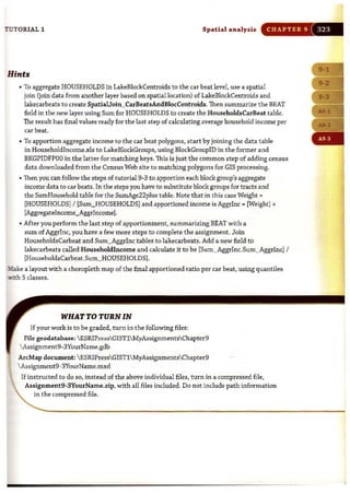
![:-DTORIAL 1
3 Type or make selections as shown in
the image at right.
4 Click OK, wait for ArcMap to finish
processing, and hide the Search
window.
5 Move BarBuffers to t he top of the
TOC and change its symbology to a
hollow fill.
Spatial analY:fi:f CHAPTER 9
' . Butler GJIQ]~
~.!I'P'I-.-L~)
!"C>..M
~L~T~{~~~..--------------
'ITC:~(~~--
8~s
I
,0 zwcoo£
D ~
...-----"1
01( II """'01 IIEtWirocment,,·· 11 Show~» I
"'"'..,.... I.. !il ........... I
D '
.. Iil·..... """""" !
•
•](https://image.slidesharecdn.com/gistutorial1basicworkbook-130505153606-phpapp01/85/Gis-tutorial-1-basic-workbook-301-320.jpg)


![CHAPTER 9 Spatial analysis
2 Type or make selections as follows:
m' . ." "' , . . .~",-_ __ _ _ __ _ _ _ _ _ _ __ __ __ __ _~
r il ~
~ +I
, ~
1 · - - - -
! ~~;;d,; ......-~
M~Rot_..'
,
-~
.±J
.,
.::.; l! ( ...:01 IjEtwr..-s.. ][ ~"",).. 1
3 ClkkOK.
YOVRTVRN
Intersect the intersection
you just created with
BufferMajorStreets to
produce BufferSuitability.
Symbolize the end
product as you wish. Turn
layers on/off as shown
in the image. Notice that
some of the suitable area
for car beat 241 is in
car beat 261. Obviously,
you would not choose
a site in the wrong car
beat. Otherwise, the
results are ready for use
for find ing sites for the
satellite police stations.
"" 1__
'" Iil ~..Cont'oo:h
•."-
"i' O ...._ _ "w...
o
10 0"'_,
o& 0 _ ....__
o
'D -o
il lil , .......
"il lil""""_
•-=============-------------------- --
GIS TU1](https://image.slidesharecdn.com/gistutorial1basicworkbook-130505153606-phpapp01/85/Gis-tutorial-1-basic-workbook-310-320.jpg)


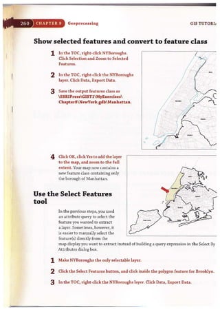
![_ TUTORIAL 1
4 In the TOe, right-dick the Surn_WeightByTract table and
dick Open. Each tract that is totally within car beats
wit: have weights sum ming to 1. Those partial1y within
car beats sum to less than 1. Check out your results by
comparing tracts on the map with tabled values.
5 Close the Attributes of Sum_WeightByTract table.
Spatial analysi.
undereducated population by car beat
This is the final step of apportionment.
CHAPTER 9 3
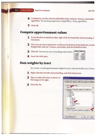
1 Open the BlockCentroidsFinal table, right-click the BEAT column heading, and click
Summarize.
2 Type or make the selections as shown in
the image at the right.
3 Click OK, Yes.
4 Right-click the Sum_UnderEducated table
in the Toe and click Open. The extra row
with no beat value is of no consequence,
because it will not join to the car beats table
in the next steps.
5 Close all open tables.
SUmmarlIC I? ,IX
til S,..,../vN
'" Ii Weight
..-o ~......
O ~......
O A"'".~
IaSum ~
o S~d 0,....
D Vorin:e
,: :0,]"
j
I](https://image.slidesharecdn.com/gistutorial1basicworkbook-130505153606-phpapp01/85/Gis-tutorial-1-basic-workbook-319-320.jpg)


![, j' m<
n system
atio - systems
-~mat.i.on systems
:Jrma ti
9;,0-;,1"_]:;11"1: '-
geographic
., f;
,n for 1!~; t. i 'Jrl
information
nformation
matio n
ation
.. "
0"
A.rcGIS 3D Analyst
SYSCr.: .,. q~G
systems geograp
systems geographic
sy ste ms ge ographic
systems geographic
stems geographic
s ge ograp h i c
phi .c
'''"''''''~
.., g eo
sys t e ms geogra phic
syste ms geographic
systems geogr'aphic
systems geographic
systems geogr'lph-' r:
:;: ." .... 1'" q . ,
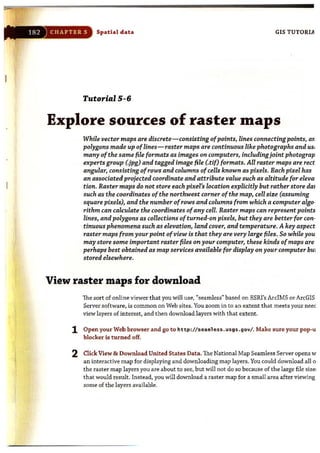
-- is chapter is an introduction to ArcGIS 3D Analyst, an extension to ArcGIS
Jesktop that enables 3D display and processing of maps. 3D viewing can
:--!,ovide insights that would not be readily apparent from a 2D map of the
id.:Ile data. For example, instead of inferring the presence of a valley from 2D
:cntours, in 3D you actually can see the valley and perceive the difference in
~ht between the valley floor and a ridge. This chapter uses topography, curb,
L--1i building data from the city of Pittsburgh's Mount Washington and Central
~ess District neighborhoods to show you how to display and analyze data
'!: 3D. It also introduces ArcGlobe, a Web service from ESRI based on 3D that
cdudes rich basemaps.
" ..- 0
l n f 0 "
in f o~
info
info
i n fo
info
in f o
info
" ,](https://image.slidesharecdn.com/gistutorial1basicworkbook-130505153606-phpapp01/85/Gis-tutorial-1-basic-workbook-328-320.jpg)


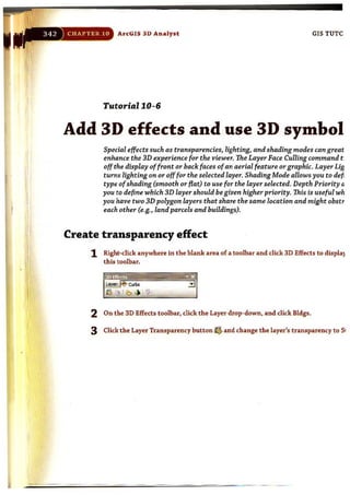
![CHAPTER 10 Arc-GIS 3D Analyst GIS TUT(
Drape buildings to TIN and extrude buildings
1 Click the Add Data button, browse to ESRIPressGISTlData3DAnalyst.gdb, an<
Bldgs and Add. This action adds the buildings layer with arbitrary heights that ArcSc
n eG-ted by default in the attribute table. Ope::l the Bldgs table to see the new Height a
2 Right-click the Bldgs layer and click Properties.
3 Click the Base Heights tab and click the radio (option) button Floating on a
custom surface.
B_H.q-t. T.... E>rt,,,,,,,,:,..
ae._from ..n0<t$
ONO...-.v....,f,""'a..n.u
~ 0 ~on. CUJlam ..nace,
fIII'r"' [C,IfsiUPr."IOISTIl't!EXOfdle$OItP:Ofllli>!toth
_~~ . HTML~
4 dick the Extrusion tab and make selections as follows:
La)"" f)ra pert,e. ~?- rxJ
:" Gcnooal ] s..... I ~ I DiIIl!or ! Jit'lJ.1II' 1" !'1Oti!- j ......... I JoN ~ IoIooIeI !
r-----a;;Ht9n f T_ 1 £.... I ....... I
--i !0EW1..de fe&n:< ., ~. E>1fusm tIIns ~. ~ _Ii re, hs "'0
.....,...-d~ rt~l*rls .
I
-
E>:tru!b> v........ _IK<IOn,
~!_l
I ~
I. I ,
1 AeIIIIr extrusion by: ..
~J
I
! ~ ltoelC!1!~on·> _ heiott ..
. r
! I
~I
•
•
I
" .. .. .... .. -
I
" II ,.... j , ~IW
...](https://image.slidesharecdn.com/gistutorial1basicworkbook-130505153606-phpapp01/85/Gis-tutorial-1-basic-workbook-337-320.jpg)


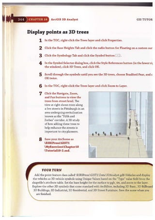


![-OTORIAL 1
YOUR TURN
Zoom in to a
mountainous area of
the globe and use the
Navigation Mode button
to see elevation. You can
view mountains in 3D.
You can find particular
mountains using Find
with the Places tab,
zooming to and then
zooming out. Then, to
view elevation, click the
01 I) ~Iorot>
·,'j "io...", I..,...,
r.; .;;. t>_,.,.,.o _ ..ood""..
D""~
Ii!~"
" -'l! !Iev...,., i<er,
Ii! I!ov"'"(""')Ii! ...,"'" (...." ..)
ArcGIS 3D Analyst
Navigation Mode button %.For instance, above is a view of Pikes Peak.
d and display large-scale vector data
CHAPTER 10
You can add and display map layers for anywhere in the world. Next, you will add two
layers for Allegheny County.
1 Click t he Add Data button; navigate to ESRIPressGISTlDataAlleghenyCounty.gdb;
hold down your Ctrl key; click CountySchools, Tracts; release the Ctrl key; and dick
Add, Finish, and Close.
2 Click t he List By Type button [ft]at the top of the TOe and drag Tracts up in the Toe
above Boundaries and Places.
3 Right-dick Tracts and dick
Zoom to Layer. You could
symbolize the tracts using
attributes in any way you wish at
this point.
4 At the top of the TOe, dick the
List By Source button .@ , right-
dick County Schools, and click
Display XY Data.
.. U m:JIII:I!II
,;, ""'''li>ro<'
I" -1 "'.....,1oy~,
... ECI ".,,,
nECI_ood .....'
Ii!I I.noo""""
1i!I _ ."
'" 'f!< I...._Iwr".
ECI £1,,,,,,,1""')
Ii!I £I'_ II'Cn/L"'1
5 Select POINT~X for the X Field; select POINT_Yfor the Y Field; and select Projected
Coordinates, State Plane, NAD 1983 (Feet), NAD 1983 StatePlane, Pennsylvania South
FIPS 3702 (Feet).prj for the projection. Click OK, Finish.](https://image.slidesharecdn.com/gistutorial1basicworkbook-130505153606-phpapp01/85/Gis-tutorial-1-basic-workbook-356-320.jpg)
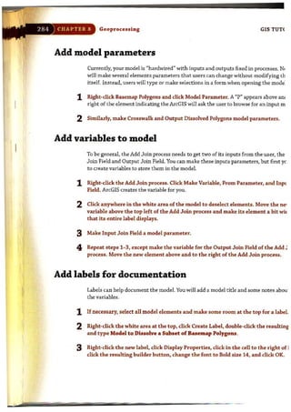
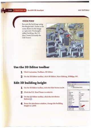
![CHAPTER 10 ArcGIS 3D Analyst
6 Turn off Tracts in the TOC, click the
Find but ton " and type or make
selections as shown in t he image at
the right.
7 Click Find and, in the resulting
bottom panel, right-click North
Allegheny High School, click Zoom
To, and close the Find window.
8 Zoom in until you see the label for
North Allegheny High School. You
can see that ArcGlobe has its own
label for the school as a pJace and
even has local streets for display.
9 Save your ArcGlobe document as
Tutoriall0-1.3dd in ESRIPress
GIST1 MyExercisesChapterlO.
YOUR TURN
GIS TUTOR
.• , ,nd
('¥.o......e'I1;;;;,.l ~
~: ~:;:~~"==-3 ~
In: F&c~~/' 3 I N"",S,
I E!lR-d fMbl'.. thot .......... toot"""",,,tho_otrhQ
1 s;:~ a
1°;:L ._ .. _.. ...-J ~
"'[] ,.....o0 -
"'_INJ_0 0 -
0 -
III DI<....eoo.Ii!l .....__,~
This Your Turn exercise has you use ArcGlobe for small-scale mapping. Start a new
ArcGlobe document by adding ESRIPressGISTlDataWorld.gdbCountry. Symbolize
Country with Quantities, Graduated colors using POP2006 normalized with SQMI (yields
persons per square mile), and quantile for classification method. When finished, do not save
your work. Close ArcGlobe. Be sure to move your Country layer above the Imagery layer.
II Q_ .....,
~~ -" oQ "'-~
'"--,~
8..""",·,,·..3IAIS-,."
1'I,,,,...zw.•
.......,....•• nc.o·~
0_""-"
0',_....
.-'" .!l .....~~
ii! _(31)0)
&!_!'OoI"-I](https://image.slidesharecdn.com/gistutorial1basicworkbook-130505153606-phpapp01/85/Gis-tutorial-1-basic-workbook-357-320.jpg)
![TUTORIAL 1 ArcGIS 3D Analyst CHAPTER 10
Assignment 10-1
Develop a 3D presentation for downtown historic
site evaluation
lhny u.s.cities, including the city of Pittsburgh, are experiencing a surge of downtown
're"ritalization. In Pittsburgh, new condominium and apartment projects are in progress, and the
dyplanning department wanh to verify that this new development does not interfere with
~ting historic sites. In this a~signment, you will help the city planning department raise the
OillRI'eness of historic sites in downtown Pittsburgh by developing a 3D model and animation of
dese areas.
.st..rtwith the following:
• ESRIPressGISTl DataAlIeghenyCounty.gdb Parks- polygon layer ofAllegheny
County Parks
• ESRIPressGISTlDataAlleghenyCounty.gdbRivers- poJygon layer of Allegheny
County rivers
• ESRIPressGISTl DataPittsburghCentraIBusinessDistric.gdbHistsite-polygon layer
of historic sites in the city of Pittsburgh's central business district
• ESRIPressGISTl Data3DAnalyst.gdb Bldgs- polygon layer of buildings in
downtown Pittsburgh
• ESRIPressGISTl 3DAnalyst.gdbCurbs- polyline layer of curbs (sidewalks) in
downtown Pittsburgh
• ESRIPressGIST1 Data3DAnalyst.gdbTopo-polyline layer of topography contours
in downtown Pittsburgh
o-te a 3D map and animation ofhistoric sites
~ a new ArcMap document called ESRIPressGISTlMyAssignmentsChapterlO
l-to""pmentlO-lYourname.mxd and add the feature classes listed above. Symbolize the features
]C'W' liking and zoom to the Bldgs layer. Create a new feature d ass of buildings that have their
ztttroid in historic sites and another of buildings whose centroids are not within historic sites
Use switch selection in the attribute table to select the nonhistoric site buildings). Save the
futures in a new file geodatabase called ESRIPressGIST1MyAssignmentsChapterlO
, -gumentlO-lYourName.gdbHistoricSiteBldgs and ESRIPressGISTlMyAssignments
_ rlOAssignmentlO-1YourName.gdb NonHistoricSiteBldgs. Remove the original Bldgs layer.
::1nArcC.1talog, create two new point features for trees and street furniture (e.g., benches, signs,
J
~:ca~ns, streetlights. etc.) in historic sites called ESRIPressGIST1 MyAssignments
lOAssignmentlO-1YourName.gdb HistoricSiteTrees and ESRIPressGISTl
.gnmentsChapterlO AssignmentlO-1YourName.gdbHistoricSiteFurniture. Assign them
same spatial reference as the historic sites (NAD_1983_StatePlane_Pennsylvania_South_
_3702_Feet). In ArcMap, digitize points representing trees and street furniture anywhere in
"""'=-st,oric site locations.](https://image.slidesharecdn.com/gistutorial1basicworkbook-130505153606-phpapp01/85/Gis-tutorial-1-basic-workbook-358-320.jpg)


![.:, '.J .
·, on sys:. Pil1S
tion sy stems
" I
g eo g('ap ."
geo.g , ap h ic
eo" r ap hic
info. m. ; tiotl .sY:' ,. "I!~S
iflfor'mation systems
i"forrllation systenlS
,,] P 1"'
ation
c'" rna t . formation syste ms
tion systems
s tern s
geogr0phic in
geographic I II
geo g l~aph ic in
ge o grap h i c in
ge ographic
ge o grap h i c
at
'.~ (. p
. ,.!T T"s yste ms
i"" ,.,,. a t:i.on systems
or illation systems
or' maliof1 systems
ol"matior' systerns
' ~form~t:iG:'1 ~;Is"'e~s
ArcGIS 'Spatial.Analyst
r ap h ic..
geographic
geogrcphic
gi?091~ap h ic
g€'ographi.:::
'PiJq"',::~h'L
," "'
-""5 chapter is an introduction to ArcGIS Spatial Analyst, an extension of
~cG IS Desktop. Spatial Analyst uses or creates raster datasets composed of
,?id cells to display data that is distributed continuously over space as a surface.
~-. this chapter you will prepare and analyze a demand surface map for the
!lxation of heart defibrillators in the city of Pittsburgh with demand based on
. ... number of out-of-hospital cardiac arrests with potential bystander help.
!":.. will also learn how to use Spatial Analyst to create a poverty index surface
";:'.a-t combines several census data measures from block and block group
?J!ygon layers.
i n
in
in
.: n
""](https://image.slidesharecdn.com/gistutorial1basicworkbook-130505153606-phpapp01/85/Gis-tutorial-1-basic-workbook-362-320.jpg)


![7UTORIAL 1 ArcGIS Spatial Analyst CHAPTER 11
:alculate predicted heart attacks
You can expect that the resulting estimate will be larger than the actual number of heart
attacks in OHCA's YES attribute, which is just a subset of all heart attacks (those in which
bystander help was possible, given the location).
1 Right-dick OHCAPredicted and open its attribute table.
2 Click Options, Add Field, and add a field called Predicted that will contain floating
point values.
3 Right-click the Predicted column beading and click Field Calculator.
4 Create the expression 5 x [RASTHRVALU] )( (Area] and click OK. OHCAdata is a five-year
sample for heart attacks, thus the expression includes the multiple 5.
5 Close the attribute table. A few of the points in OHCA have no raster values near them,
so ArcGIS assigns the value - 9999 to them to signify missing values. Before looking at
a scatter plot of predicted and actual values, you will first select only OHCA points with
positive predicted values.
6 Click Selection, Select by Attributes.
7 For the OHCAPredicted layer, create the expression "Predicted" )= 0 and click OK.
8 Right-click OHCAPredicted, and click Data and Export Data.
9 Export selected features to ESRIPressGISTlMyExercisesChapterl1
OHCAPredicted2.shp and click Yes to add the shapefile to the map.
10 Clear the selected features and turn off the OHCA_Predicted layer.](https://image.slidesharecdn.com/gistutorial1basicworkbook-130505153606-phpapp01/85/Gis-tutorial-1-basic-workbook-374-320.jpg)


![=
380 CHAPTRR 11 ArcGIS Spatial Analyst GIS TUTORIAL :
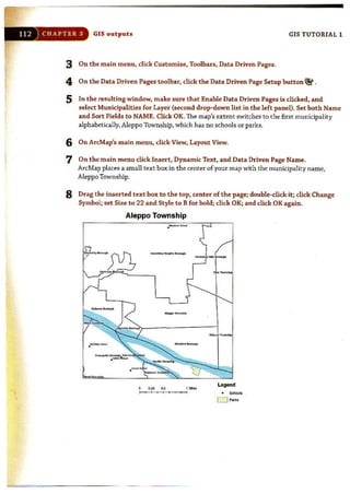
2 On the main menu, dick Geoprocessing,
Geoprocessing Options, and make
selections as shown in the image at
the right.
-,0 ~ tho oo.t.pW <i _oces<in9_oI:lcn<
0Log_oce'<in9_lltionsto~lo.;lfloI "
e.u..;,oo.rd 1'1"".---.. .....
3 Click OK. .--J - - _ .-
4 On the main menu,click Geoprocessing,
Environments, Raster Analysis, and
Select As Specified Below for Cell Size.
Type 150 for the specification, select
Pittsburgh for the Mask, and click OK.
5 Save the map document in ESRIPress
GISTlMyExercisesChapterll. I~
0iIpI0y I T",-MY ~
0 Addradsd~*'CI_NiM$ to""~
O~'or.t._",ybydefld "
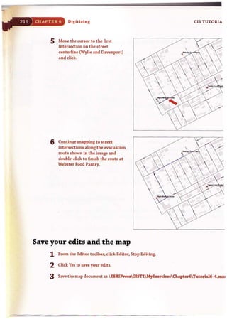
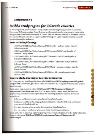
Standardize input variables
Here you will calculate the z-score in an attribute table of one of the input feature classes.
To save time, the other three variables already have z-scores ready for use.
1 Right-dick AlICoBlocks in the TOe and click Open Attribute Table.
2 Scroll to the right, right-click FHHChld, and click Statistics. It is convenient to copy and
paste the statistics to Notepad and then copy and paste them later to the field calculator
that you will use.
3 On your desktop, click Start, All Programs, Accessories, Notepad.
4 Select all of the statistics in the Statistics of
AllCoBlocks window, pres Ctrl+C, click inside the
Notepad window, and press Ctrl+V.
5 Close the Statistics of AllCoBlocks window,
click the Table Options button ~ .. in the Table
window, dick Add Field, type ZFHHChld for
Name, select Float for Type, and click OK.
~.. .Edit FOrll'lll VItW ~
Count: - 2428 f - ~-~=~
Minimum: 0
~a ximum: 186
Sum: 34534
Mean: 1.422147
Standard Deviation: 4.431102
6 Right-click the column heading for ZFHHChld, click Field Calculator, and create the
following expression in the bottom panel of the Field Calculator window by copying
and pasting from your Notepad window,:
( [FHHChld] - 1.422147) 1 4 .431302](https://image.slidesharecdn.com/gistutorial1basicworkbook-130505153606-phpapp01/85/Gis-tutorial-1-basic-workbook-383-320.jpg)

![-
CHAPTER 11 ArcGIS Spatial Analyst GIS TUTOR]
4 Type or make the selections as
shown in the image at the right.
5 ClickOK.
6 Right-click the Kernel Density
tool element, click Rename,
and change the name to
FHHChld Kernel Density.
7 Right-click FHHChld Kernel
Density and click Run.
" tHH[ hid I«,.oll)o."'y
8 Right-click the KDFHHChld and click Add to Display.
YOUR TURN
'1 I.
Resymbolize the new layer using the Classified method with 1/4 standard deviations and
the color ramp that runs from blue to yellow to red. Turn off the point feature layers. The
result is as follows:
." L.,....
.. 0 ctiGA
" O'l "''"D
"' 0 .0>0::_
~ 0 ""''''''''''
,.""""D
Ii< O'l ''''''''~
<"I"''",. 0·0."""" "'". o,ooooo"m _o,oco:"'o"
;;,."""'..,.. -o,ocooo","
ID o,O>:W035 ·O,ocm:0021
8 0,,,,,,",,,,, ' . 0,"""'110"
D O,ro:", Loo, _, ,ocwt4,...
Co."""',....-0."""'1''''Do,,,,,,,,,,,,,.-0."""" '''''
0 0,"""',,,,,,·,."""''''''''B ' ,ro:o:z=o _'.0C002'5IJ5
lIlIo,,,,,,,,,,""'-o,,,,,,,,m,,
m o,,,,,,",ml - o,roJO>]"'"
. 0,oo:m:tJ93· , ."""""""
. 0,,",,,,,,,,,'_0."""''''''''. o,""""''''_'_'''''L'''''''
Create a kernel density layer for a second input
il l
You can reuse the model elements you just built. While blocks work very well with a se,
radius of 1,500 feet, there are fewer block groups (the remaining three poverty inputs
at the block group level), so you need a larger search radius of 3,000 feet for them.](https://image.slidesharecdn.com/gistutorial1basicworkbook-130505153606-phpapp01/85/Gis-tutorial-1-basic-workbook-385-320.jpg)


![I
CHAPTER 11 ArcGIS Spatial Analyst
WHAT TO TURN IN
If your work is to be graded, turn in the following files:
ArcMap document: ESRIPressGISTlMyAssigmentsChapter11
Assignment11-2YourNarne.mxd
File geodatabase: ESRIPressGIST1MyAssigmentsChapterll
Assignment11-2YourNarne.gdb
If instructed to do so, instead of the above individual files, turn in a compressed
GIS TUTOR]
file, Assignment11-2YourName.zip, with all files included. Do not include path information
in the compressed file.](https://image.slidesharecdn.com/gistutorial1basicworkbook-130505153606-phpapp01/85/Gis-tutorial-1-basic-workbook-393-320.jpg)


![liS TUTOR1AL 1
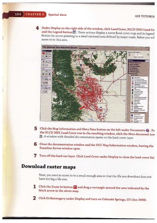
l Accept the default installa-
tion folder or click Browse
and navigate to the drive or
folder location where you
want to install the data.
Click Next. The installation
will take a few moments.
When the installation is
complete, you will see the
following message.
Installing tb. data and sof'twar. APPENDIX D
l.;t GIS 1utOrlal 1 Student R('S()llrH'~ In..tall$hleld WIzard rg)
Destination folder
.-
O !N ~ GIS Tutorillll·Student I!.HOU"Ce'lto:
C:'ES!l.lPreSll
~'"
<~d n Next > 1I CMet!
1& <iIS Tlltorial 1 . Student Resourc~ InstallShield WIzard [EJ
1115tallShleld Wiza rd Completed
Th! tnslalShleld ",l:¥d .....s ,••n~sfuly instaled GIS T~toriaI I
. S~I Re5cuces. CId: Art$!] to exit !he .'lizard.
Click Finish. The exercise data is installed on your computer in a folder called
C:ESRIPressGIST1.](https://image.slidesharecdn.com/gistutorial1basicworkbook-130505153606-phpapp01/85/Gis-tutorial-1-basic-workbook-414-320.jpg)


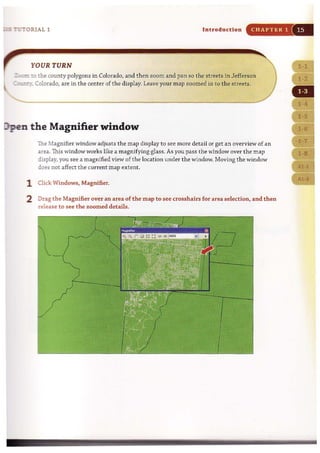
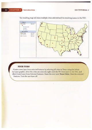
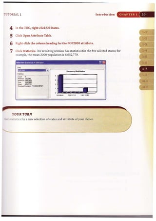
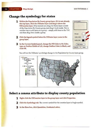
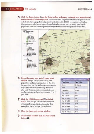
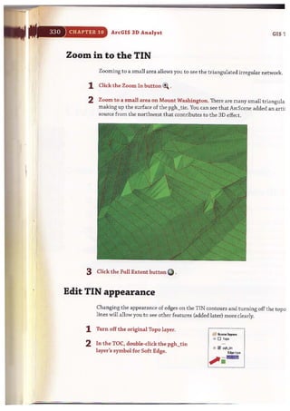
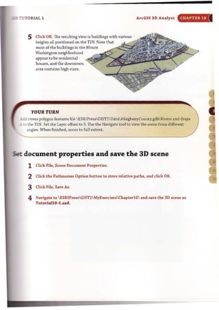
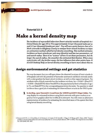
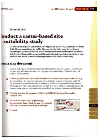
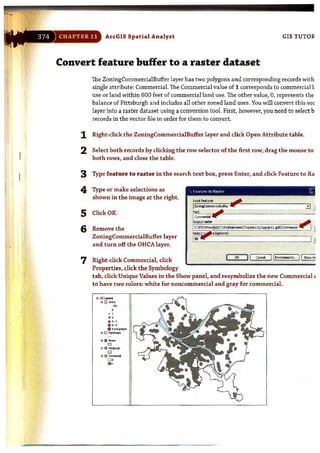
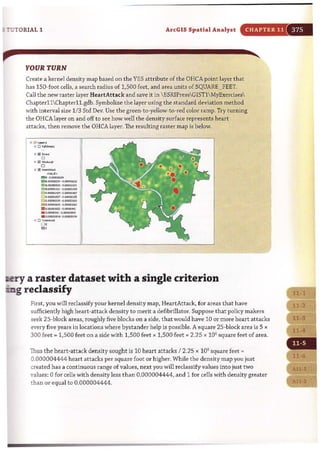
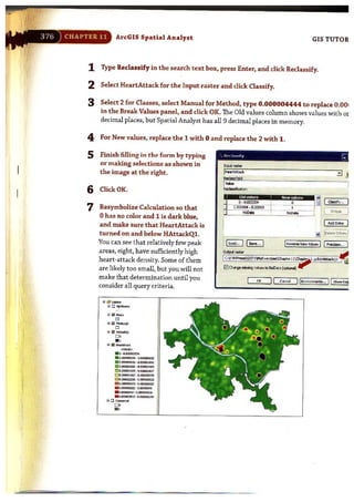
This tutorial familiarizes you with some basic features of ArcGIS and illustrates fundamentals of GIS. You will work with map layers and underlying attribute data tables for U.S. states, cities, counties, and streets. You will open an existing map document, save it to a new location, and learn how to work with map layers, navigate maps, measure distances, work with feature attributes, select features, and work with attribute tables. The goal is to introduce basic GIS concepts and skills.


