Edge Detection
• Indigital image processing edges are places where the brightness or
color in an image changes a lot.
• These changes usually happen at borders of objects.
• Detecting edges helps us understand the shape, size and location of
different parts in an image.
• Edge detection is used to recognize patterns, understand image
structure and pick out important features in images.
3.
Types of EdgeDetection Operators
• There are two types of edge detection methods:
1. Gradient-Based Edge Detection Operators
• Gradient-based operators detect edges by measuring how quickly the pixel values or brightness changes in a image.
• These changes are called gradients.
• If the change is large between two neighboring pixels that indicates an edge. They use first derivative to find edges.
2. Gaussian-Based Edge Detection Operators
• Gaussian-based operators combine blurring and edge detection.
• They reduce the effect of noise by smoothing the image first and then look for changes using the second derivative.
• These are more advanced and accurate than gradient-based operators.
5.
Sobel Operator
• TheSobel Operator is a method used to detect edges in an image by checking
how pixel values (brightness) change in the horizontal and vertical directions.
• It uses two 3 x 3 kernels or masks which are convolved with the input image to
calculate the vertical and horizontal derivative approximations respectively:
where:
• Mx detect edges from left to right
• My detect edges from top to bottom
• By combining the results from both it finds the overall edge strength and
direction.
6.
Prewitt Operator
• Itis very similar to the Sobel Operator but with slight difference is that it calculates
the edge gradients.
• Like Sobel it detects edges in the horizontal and vertical directions using two 3×3
matrices but it uses a uniform averaging technique in its kernel making it less
accurate than Sobel but faster and simpler to implement.
where:
• Mx detect edges from left to right
• My detect edges from top to bottom
• By combining the results from both it finds the overall edge strength and direction.
7.
Roberts Operator
• Itis one of the simplest edge detection methods as it focuses on how
pixel values change diagonally in an image.
• The operator uses a 2×2 kernel to calculate the gradient of intensity
between diagonally adjacent pixels and make it suitable for detecting
edges that appear along diagonal directions.
• n matrix algebra, the symbols Mxand Mycan represent specific
transformation matrices, such as those for reflections or rotations.
The matrices you provided are:
• Mx is a 2x2 matrix that can represent a reflection across the x-axis.
The matrix is given as:
8.
• My isa 2x2 matrix that can represent a rotation by 90 degrees
clockwise around the origin. The matrix is given as:
• Applying this matrix to a vector (x,y) transforms it to (−y,x), which is
the result of a 90° clockwise rotation.
• Mx detects diagonal edges that run from top-left to bottom-right.
• My detects diagonal edges that run from top-right to bottom-left.
• By combining the results of both kernels the Roberts operator
calculates the gradient magnitude to highlight edges.
9.
Marr-Hildreth Operator orLaplacian of Gaussian (LoG)
• Marr-Hildreth Operator is also called Laplacian of Gaussian (LoG) and
it is a Gaussian-based edge detection method.
• It works by first smoothing the image using a Gaussian filter to
remove noise and then applying the Laplacian operator to detect
regions where the intensity changes sharply.
• The LoG operator first smooths the image using a Gaussian filter to
reduce noise then applies the Laplacian to detect edges.
• It detects edges at zero-crossings where the result changes from
positive to negative.
10.
Where:
• σ =standard deviation of the Gaussian filter
• x,y = pixel coordinates
• Use LoG when your image is noisy and you need clean it.
11.
Canny Edge Detector
•The Canny operator is one of the most advanced and widely used
edge detection methods.
• It uses a multi-step process to detect sharp and clean edges while
minimizing noise.
1. Noise Reduction using Gaussian Blurring:
Before detecting edges, we remove noise using a Gaussian Blur and
smoothens the image.
2. Find Intensity Gradient: In this step we find where the image
changes the most this helps detect edges. We use Sobel filters to find
gradients in x and y directions:
12.
3. Non-Maximum Suppression:We thin the edges
by keeping only the local maximum gradient in the
direction of the edge. It removes pixels that are not
part of a strong edge.
4. Double Thresholding: Here we classify pixels into:
• Strong edges (above high threshold)
• Weak edges (between low and high threshold)
• Non-edges (below low threshold)
4. Edge Tracking by Hysteresis: The final step
connects weak edges to strong edges if they are
part of the same structure. Isolated weak edges are
removed.
13.
Corner and InterestPoint Detection
• Corner and interest point detection are fundamental techniques in
computer vision used to identify distinctive points in images that can
be reliably located and matched across different views or
transformations.
• These points, often found at the intersection of edges, are crucial for
various applications like image registration, object recognition, and
scene understanding.
• These points, often found at the intersection of edges, are crucial for
various applications like image registration, object recognition, and
scene understanding.
14.
Key Concepts:
Corners asInterest Points:
• Corners are a specific type of interest point characterized by
significant intensity changes in multiple directions. They are more
distinctive than edges, making them ideal for feature detection.
Interest Points:
• Interest points are locations in an image that are easily detectable and
remain relatively stable under geometric and photometric
transformations (like rotation, scaling, and illumination changes).
15.
Applications:
• Corner andinterest point detection are used in numerous computer
vision tasks, including:
• Image Registration: Finding corresponding points between images to align
them accurately.
• Object Recognition: Identifying and recognizing objects based on their
distinctive features.
• Motion Detection: Tracking the movement of objects by detecting changes in
their location over time.
• Panorama Stitching: Creating panoramic images by combining multiple
overlapping images.
• 3D Reconstruction: Reconstructing the 3D structure of a scene from multiple
2D images.
• Image Retrieval: Searching for images based on their feature content.
16.
Corner Detection Methods:
•Harris Corner Detector: A widely used algorithm that computes a
corner response function based on the eigenvalues of a structure
tensor. It identifies corners as points where both eigenvalues are
large.
• Shi-Tomasi Corner Detector: Similar to Harris, but it uses a different
corner response function, often leading to better performance in
some cases.
• SUSAN Corner Detector: Uses a mask to count pixels with similar
brightness to the center pixel and identifies corners based on a
threshold.
17.
Interest Point Detectors:
•SIFT (Scale-Invariant Feature Transform): A popular detector that
finds interest points at multiple scales and computes scale-invariant
descriptors.
• SURF (Speeded-Up Robust Features): Another scale-invariant
detector that is faster than SIFT.
• ORB (Oriented FAST and Rotated BRIEF): A fast detector and
descriptor that combines the FAST corner detector and BRIEF
descriptor.
18.
Key Attributes ofInterest Points:
• Rich Image Content: The area surrounding an interest point should
contain significant information.
• Well-Defined Representation: An interest point should have a
descriptor that can be used for matching.
• Well-Defined Position: The location of the interest point should be
precise.
• Invariance: Interest points should be robust to changes in rotation,
scaling, and illumination.
• Repeatability: The same interest points should be detected in
different views of the same scene.
19.
Image Segmentation
• Imagesegmentation is a key task in computer vision that breaks down
an image into distinct, meaningful parts to make it easier for
computers to understand and analyze.
• By separating an image into segments or regions based on shared
characteristics like color, intensity or texture, it helps identify objects,
boundaries or structures within the image.
• This allows computers to process and interpret visual data in a way
that’s similar to how we perceive images.
• The process involves grouping pixels with similar features, assigning
labels to each pixel to indicate its corresponding segment or object
and generating a segmented image that visually highlights the
different regions.
20.
Why do weneed Image Segmentation?
• Image segmentation breaks down complex images into smaller,
manageable parts making analysis more efficient and accurate. By
separating objects from the background, it allows for deeper
understanding of the image.
• This is important for tasks like:
• Self-driving cars: Detecting pedestrians, vehicles and road signs.
• Medical imaging: Analyzing scans for tumors organs or abnormalities.
• Object recognition: Identifying specific items in various fields like retail or
wildlife monitoring.
• Automation: Helping robots navigate and interact with their environment.
21.
Types of ImageSegmentation
• Image segmentation can be categorised into three main types based on the
level of detail and the tasks being performed:
1. Semantic segmentation:
• It involves assigning a class label to every pixel in an image based on shared
characteristics such as colour, texture and shape.
• This method treats all pixels belonging to the same class as identical,
without distinguishing between individual objects.
• Example:
• In a street scene: all pixels of "road" are one label, all "cars" are another, all "people"
are another.
• Example image (semantic segmentation):
• Input: A photo of a street.
• Output: Road pixels → gray, cars → blue, pedestrians → green.
22.
2. Instance segmentation:
•Instance Segmentation extends semantic segmentation by not only labelling colour of each pixel
but also distinguishing between individual objects of the same class.
• This approach identifies each object of the same class as a unique instance.
• Example:
• In a street photo with 3 cars → each car is highlighted with different colors.
• Input: Image of 3 cats.
• Output: Cat-1 → red mask, Cat-2 → blue mask, Cat-3 → green mask.
3. Panoptic segmentation:
• Panoptic segmentation combines both semantic and instance segmentation techniques, providing
a complete image analysis.
• It assigns a class label to every pixel and also detects individual objects.
• This combined approach helps us to understand both broad categories and detailed object
boundaries simultaneously.
• Example:
• In a traffic image:
• All “road” pixels → one class (semantic).
• Each car/pedestrian → separately outlined (instance).
23.
Techniques of ImageSegmentation
Let's see various techniques used in image segmentation:
Thresholding: This method involves selecting a threshold value and classifying
image pixels between foreground and background based on intensity values.
• Example:
• Medical X-ray: Tumor region (white pixels above threshold), background (black).
• Methods: Global, Adaptive, Otsu’s.
Edge Detection: It identify abrupt change in intensity or discontinuation in the
image. It uses algorithms like Sobel, Canny or Laplacian edge detectors.
Example: Canny detector used in license plate recognition (edges of numbers/letters
extracted).
Region-based segmentation: This method segments the image into smaller regions
and iteratively merges them based on predefined attributes in color, intensity and
texture to handle noise and irregularities in the image.
Example: Satellite image: Separate water bodies, forest, and urban areas based on
color similarity.
24.
• Clustering Algorithm:This method uses algorithms like K-means or
Gaussian models to group object pixels in an image into clusters
based on similar features like colour or texture.
• Example:
• In a fruit basket photo, K-means can separate apples, bananas, and
oranges based on color.
• Watershed Segmentation: It treats the image like a topographical
map where the watershed lines are identified based on pixel intensity
and connectivity like water flowing down different valleys.
• Example:
• Microscopic cell images: Watershed separates overlapping cells into
distinct boundaries.
25.
Thresholding Based Segmentation
•Thresholding is a simple yet fundamental image segmentation technique
that converts a grayscale image into a binary image by comparing pixel
intensities to a threshold value.
• Pixels above the threshold are typically assigned to one class (e.g.,
foreground), while those below are assigned to another (e.g.,
background).
• This method is effective when there's a clear contrast between the
objects of interest and the background.
26.
How Thresholding Works:
1.Gray-scale Image:
• Thresholding operates on a grayscale image, where each pixel has an intensity value,
typically ranging from 0 (black) to 255 (white).
2. Threshold Value:
• A threshold value is chosen (either manually or automatically).
3. Pixel Classification:
• Each pixel is compared to the threshold. If its intensity is greater than the threshold, it's
classified as belonging to the foreground (often represented as white or 1), and if it's less
than or equal to the threshold, it's classified as background (often represented as black
or 0).
4. Binary Image:
• The result is a binary image, where each pixel has one of two values, representing the
segmented objects and the background.
27.
Types of ThresholdingMethods:
• Global Thresholding: Uses a single threshold value for the entire
image.
• Adaptive Thresholding: Uses different threshold values for different
regions of the image, often based on local image characteristics.
• Otsu's Method: An automatic threshold selection method that finds
the optimal threshold by maximizing the variance between the two
classes (foreground and background).
• Kittler-Illingworth Method: Another automatic method that
minimizes the within-class variance to find the best threshold.
• Maximum Entropy Method: Selects the threshold that maximizes the
entropy of the segmented regions.
28.
Advantages of Thresholding:
•Simplicity: It's a straightforward and easy-to-implement
technique.
• Computational Efficiency: It requires relatively low
computational power.
• Fast Processing: Can be used for real-time applications.
29.
Limitations of Thresholding:
•Sensitivity to Noise and Illumination:
Thresholding can be sensitive to noise and variations in
lighting, which can affect the accuracy of segmentation.
• Not Suitable for Complex Images:
It may not be effective for images with uneven lighting or
complex textures.
• Single Threshold:
May not be sufficient for segmenting images with multiple
objects or varying intensities.
30.
Examples of ThresholdingApplications:
• Medical Imaging: Segmenting organs or tumors in medical scans.
• Optical Character Recognition (OCR): Separating text from the background.
• Object Detection: Identifying objects of interest in images.
• Industrial Inspection: Detecting defects or anomalies in manufactured
products.
31.
Region-based segmentation
• Indigital image processing divides an image into distinct regions based
on similarity criteria.
• It focuses on grouping pixels with similar characteristics, unlike edge-
based methods that focus on boundaries.
• This approach aims to simplify the image by representing it as a set of
meaningful regions that correspond to objects or parts of objects.
• Applications
• Finding tumors, veins, etc. in medical images
• Finding targets in satellite/aerial images,
• Finding people in surveillance images etc.
• Methods: Thresholding, K-means clustering, etc.
33.
Common Techniques:
Region Growing:
•Procedure of grouping pixels or sub regions into larger regions.
• Starts from a "seed" pixel and iteratively adds neighboring pixels with
similar properties until a certain threshold is met.
• Region growing based techniques are better than the edge-based
techniques in noisy images where edges are difficult to detect.
34.
Advantages
Region growing methodscan correctly separate the regions that the
same properties we define.
• Region growing methods can provide the original images which have
clear edges with good segmentation results.
• The concept is simple. We only need a small no.of seed points to
represent the property we want, then grow the region.
Disadvantages
• Computationally expensive.
• It is a local method with no global view of the problem.
• Sensitive to noise.
35.
Region Splitting
• Regiongrowing starts from a set of seed points.
• An alternative is to start with the whole image as a single region and
subdivide the regions that do not satisfy a condition of homogeneity.
Region Merging
• It is the opposite of region splitting.
• Start with small regions (e.g., 2x2 or 4x4 regions) and merge the
regions that have similar characteristics (such as gray level, variance);
• Typically, splitting and merging approaches are used iteratively.
37.
Advantages
• Handles noisyimages well:
Region growing, in particular, can be effective in images with noise
where edges are difficult to detect.
• Can be robust to variations in lighting:
Adaptive thresholding methods can be used to account for varying
lighting conditions across the image.
• Provides meaningful regions:
The resulting regions often correspond to objects or parts of objects,
making them useful for subsequent analysis.
38.
Disadvantages
• Computationally expensive:
Someregion-based methods, like region growing, can be
computationally intensive, especially for large images.
• Sensitive to noise:
Noise can lead to over-segmentation (too many small regions) or
under-segmentation (regions not properly separated).
• Requires careful selection of parameters:
The choice of similarity criteria and thresholds can significantly impact
the segmentation results.
39.
• Clustering Algorithm:This method uses algorithms like K-means or
Gaussian models to group object pixels in an image into clusters
based on similar features like colour or texture.
• Example:
• In a fruit basket photo, K-means can separate apples, bananas, and
oranges based on color.
K-means Clustering
• K-means is an iterative, unsupervised algorithm that partitions data
points into a predefined number of clusters, denoted by 'k’.
• It aims to minimize the sum of squared distances between data
points and their assigned cluster centroids.
40.
Example: Image Segmentation
•Imagine an image of a red apple on a green leaf. We can use K-means to separate the apple
from the leaf.
• Define 'k': We know we want to separate the apple (one cluster) from the leaf (a second
cluster). So, we set k = 2.
• Initialization: The algorithm randomly picks two pixels from the image to act as the initial
cluster centers (centroids) for 'apple' and 'leaf'. Let's say one pixel is a random shade of red
and the other is a random shade of green.
• Assignment: The algorithm goes through every single pixel in the image. It looks at a pixel's
color and assigns it to the closest centroid. A dark red pixel would be assigned to the 'apple'
centroid, while a light green pixel would be assigned to the 'leaf' centroid.
• Update: After all pixels are assigned, the algorithm recalculates the new 'apple' centroid by
averaging the colors of all pixels assigned to it. It does the same for the 'leaf' centroid.
• Iteration: The process repeats, with pixels being reassigned to the new, more accurate
centroids. This continues until the centroids stop moving. The final result is an image where
all the 'apple' pixels are one solid color (the final centroid color) and all the 'leaf' pixels are
another solid color.
41.
Application in ImageProcessing:
• K-means is widely used for image segmentation by clustering pixels
based on their color or intensity values, grouping similar pixels into
distinct regions.
42.
Mean Shift Clustering
•Mean Shift is a non-parametric, unsupervised clustering algorithm
that identifies clusters by iteratively shifting data points towards the
modes (densest regions) of the data distribution.
• It does not require a pre-defined number of clusters.
• Example: Image Segmentation
• Let's use the same image of the red apple on a green leaf.
• Initialization: For each data point, define a window (e.g., a circular or
spherical kernel) around it.
• Mean Shift Vector Calculation: Calculate the mean of the data points
within the window. The difference between this mean and the current
data point's position is the mean shift vector.
43.
• Shifting: Shiftthe data point in the direction of the mean shift vector.
• Iteration: Repeat steps 2 and 3 until the data point converges to a mode (a
local peak in the density function).
Application in Image Processing:
• Mean Shift is effective for image segmentation, particularly for handling
irregularly shaped clusters and determining the number of segments
automatically. It is also used in object tracking and feature extraction.
44.
Comparison in ImageProcessing:
• K-means:
Simpler and faster, but requires 'k' to be specified beforehand and may
struggle with non-globular or overlapping clusters.
• Mean Shift:
More flexible as it doesn't require pre-defining 'k' and can discover
arbitrarily shaped clusters. However, it can be computationally more
expensive and sensitive to the bandwidth parameter.
45.
Morphological image processing:Erosion and
Dilation
• Morphological operations are image-processing
techniques used to analyze and process
geometric structures in binary and grayscale
images.
• These operations focus on the shape and
structure of objects within an image. They are
particularly useful in image segmentation,
object detection, and noise removal tasks.
• Erosion shrinks objects, while dilation expands
them, both using a structuring element to
define the extent of the change.
• These operations are crucial for noise reduction,
object separation, and feature extraction.
46.
Erosion
Purpose:
• Reduces thesize of objects in an image by removing pixels from their
boundaries.
How it works:
• The structuring element acts as a "probe" that slides over the image.
• If the structuring element fits entirely within the object at a given location,
the corresponding pixel in the output image remains the same.
• If any part of the structuring element extends beyond the object, the
corresponding pixel in the output is set to background.
Effects:
• Erodes away small details, breaks connections between objects, and can be
used to eliminate noise.
47.
Dilation:
Purpose:
• Increases thesize of objects in an image by adding pixels to their
boundaries.
How it works:
• The structuring element slides over the image, and if any part of the
structuring element overlaps with an object, the corresponding pixel
in the output is set to the object's value.
Effects:
• Enlarges objects, fills in small holes and gaps, and can be used to
connect broken parts of an object.
48.
Opening
• A two-stepprocess: erosion followed by dilation, using the same structuring
element.
• Primarily used to remove small objects, noise, and thin protrusions from an
image.
• Preserves the general shape and size of larger objects while removing smaller
ones.
• Think of it as "opening" up narrow passages or gaps in objects.
Closing:
• A two-step process: dilation followed by erosion, using the same structuring
element.
• Primarily used to fill small holes and gaps within objects, as well as smoothing
their contours.
• Preserves the general shape and size of larger objects while filling small holes.
• Think of it as "closing" up small gaps or holes within objects.
49.
Structuring Element
• Botherosion and dilation rely on a structuring element, which is a small shape (e.g., a circle,
square, or line) used to probe the image.
• The choice of structuring element significantly impacts the results of erosion and dilation.
Applications
Noise Reduction:
• Erosion can remove small, isolated noise spots, while dilation can fill in small holes caused by
noise.
Object Separation:
• Erosion can help separate connected objects by breaking narrow bridges, while dilation can fill
in small gaps between objects.
Feature Extraction:
• Dilation can be used to emphasize the boundaries of objects, highlighting their shapes.
Image Analysis:
• Erosion and dilation are fundamental building blocks for more complex morphological
operations.
51.
• Original Image:This is the starting point—a grayscale image of a lake
with mountains and a sunrise.
• Erosion: This process "shrinks" or "thins" the bright areas (or "grows"
the dark areas). You can see that the bright sunburst in the sky and
the reflections on the water appear slightly smaller and less defined
compared to the original image.
• Dilation: This is the opposite of erosion. It "grows" or "thickens" the
bright areas (or "shrinks" the dark areas). In this image, the bright
sunburst and the reflections on the water look a little larger and more
pronounced.
52.
• Opening: Thisoperation is an erosion followed by a dilation. The key
purpose of opening is to remove small, bright "islands" or noise and
smooth the contours of objects. Notice how some of the smaller,
brighter details are gone, but the overall shape of the brighter parts is
more or less preserved.
• Closing: This operation is a dilation followed by an erosion. It is used
to close small holes and gaps in bright areas and connect separate
bright objects. In this image, the bright areas seem a bit more solid
and connected, and any small dark gaps within them have been filled
in.
53.
Applications in shapeanalysis
• Shape analysis in image processing is a critical field that
involves the extraction, description, and analysis of
geometric properties of objects within digital images.
• By quantifying and characterizing an object's shape, this
technique enables a wide range of applications across
various industries.
54.
• Medical Imaging
Inmedical imaging, shape analysis is used for diagnosing diseases and
planning treatments. It helps in:
Tumor Detection and Characterization: By analyzing the shape and
boundaries of suspicious growths, doctors can distinguish between benign
and malignant tumors. The compactness, circularity, and irregularities of a
tumor's shape provide valuable diagnostic information.
Anatomical Modeling and Analysis: Shape analysis is used to create 3D
models of organs and other anatomical structures from medical scans (like
MRI or CT). This helps doctors study changes in shape related to illnesses or
developmental disorders and is also vital for surgical planning.
Cell Morphology: Researchers use shape analysis to study the shape of
cells, which can indicate disease. For example, the shape of red blood cells
can be analyzed to diagnose conditions like sickle cell anemia.
55.
Object Recognition andSurveillance
• Shape analysis is a fundamental component of many object recognition
systems. It allows computers to identify and classify objects based on their
outlines and forms.
• Vehicle Classification: In traffic management and surveillance, shape analysis
can classify vehicles (e.g., cars, trucks, motorcycles) from images or video
streams by analyzing their silhouettes.
• Biometric Recognition: Face recognition and fingerprint analysis use shape-
based features. The unique geometric features of a person's face or the
distinct patterns of ridges in a fingerprint are analyzed and matched against a
database.
• Industrial Automation: In manufacturing, robots use shape analysis to
identify, sort, and manipulate parts on an assembly line. This ensures correct
parts are used and helps with quality control by detecting defects in a
product's shape.
56.
Environmental and ScientificAnalysis
Shape analysis extends beyond man-made objects to a variety of
natural and scientific applications.
• Geology and Particle Analysis: It can be used to analyze the shape of
grains in a rock sample to determine its origin and properties. In
manufacturing, it's used to analyze the size and shape distribution of
particles in powders.
• Archaeology and Paleontology: Archaeologists use shape analysis to
match fragments of pottery or other artifacts, helping them
reconstruct historical objects. Similarly, paleontologists can analyze
the shape of fossilized bones to understand the morphology of
ancient species.
57.
Texture
• In thecontext of image processing and computer vision, it's defined as the
spatial arrangement and variation of pixel intensities (or colors).
• It helps describe the "feel" or "look" of an object's surface in an image, such
as whether it's coarse, smooth, rough, or bumpy, and it's a key feature used
to identify patterns and structures that color or shape alone can't capture.
• Purpose of Texture Analysis
•
The purpose of texture analysis is to quantify and characterize the textural
properties of a material or an image.
• This is done by measuring various features like contrast, coarseness, and
directionality.
• By converting these subjective qualities into objective, numerical data,
texture analysis enables a wide range of applications across different fields.
63.
• 1. InputImage
•
The process starts with an Input Image. This is the raw, digital image that contains
the textures you want to analyze and classify.
• The image could be anything from a photograph of a fabric to a medical scan, and
it's the subject of all subsequent processing.
2. Filtering
The next step is Filtering. This stage applies a filter to the input image to enhance or
extract specific features related to texture.
Filtering techniques can include:
Gabor filters: These are particularly effective for analyzing texture because they can
capture features at different scales and orientations, similar to how the human visual
system works.
Wavelet transforms: These decompose the image into different frequency sub-
bands, allowing for the analysis of textures at various resolutions.
The goal of this
step is to make the textural patterns more distinct and easier to analyze in the later
stages.
64.
3. Smoothing
•
Afterfiltering, the image is passed through a Smoothing step.
Smoothing is a process used to reduce noise and unwanted high-
frequency content in the image.
• This can be done using techniques like:
•
Averaging filters: These replace each pixel's value with the average of
its neighboring pixels, which blurs the image and reduces sharp,
random variations (noise).
•
Gaussian filters: These use a weighted average, giving more
importance to pixels closer to the center, which results in a smoother,
more natural-looking blur.
Smoothing helps to clean up the data and
prepares it for the final classification step by creating more uniform
regions of texture.
65.
4. Classifier
• TheClassifier is the core of the texture classification system. At this stage, a machine learning
algorithm is used to analyze the processed image data and categorize each pixel or region into a
specific texture class.
• The classifier uses the information gathered from the filtering and smoothing steps to make a
decision. Common classifiers used in this context include:
• Support Vector Machines (SVM): A supervised learning model that finds the optimal hyperplane
to separate data points into different classes.
Neural Networks: These models can learn complex
patterns and are highly effective for image classification tasks.
•
K-Nearest Neighbors (KNN): A simple algorithm that classifies a data point based on the majority
class of its 'k' nearest neighbors.
The classifier's job is to assign a label (e.g., "wood," "brick,"
"grass") to each part of the image.
5. Segmented Image
The final output is the Segmented Image. This image is the result of the
classifier's work. Instead of a single, continuous picture, the segmented image is divided into
distinct regions, where each region is labeled with its corresponding texture class. For example, in
a picture of a lawn with a sidewalk, the segmented image would clearly delineate the "grass"
region from the "concrete" region. This final output is useful for a wide range of applications, from
medical image analysis to remote sensing and quality control in manufacturing.
67.
Applications:
• Texture analysisis used in a wide range of fields, including:
• Object Recognition: Identifying objects based on their textural
features.
• Medical Imaging: Analyzing tissue characteristics and identifying
abnormalities.
• Materials Science: Characterizing the structure and properties of
materials.
• Surface Defect Detection: Finding imperfections on surfaces.
• Remote Sensing: Analyzing land cover types and geological
formations.
68.
Common Approaches:
1. StatisticalMethods:
• Gray-Level Co-occurrence Matrices (GLCM): Analyze the statistical
relationships between pixel intensities at different spatial lags.
• Run-Length Matrices (RLM): Characterize texture based on the length of
runs of consecutive pixels with the same intensity.
• Other Statistical Measures: Mean, variance, entropy, and other statistical
properties of the image histogram or local regions.
2. Structural Methods:
• Texture Elements (Texels): Identify repeating patterns or primitives (like
bricks in a wall) and analyze their arrangement.
• Structural Relationships: Define the rules for how Texels are placed
together to form the overall texture.
69.
3. Spectral Methods:
•Fourier Transform: Analyze the frequency components of the image
to detect periodicity and dominant orientations.
• Wavelet Transform: Decompose the image into different frequency
bands to capture texture features at various scales.
4. Model-Based Methods:
• Fractals: Use fractal geometry to model the self-similar nature of
textures.
• Markov Random Fields (MRF): Model the spatial dependencies
between pixels using probabilistic methods.
70.
• 1. StatisticalMethods (Texture Analysis)Statistical methods describe texture by measuring
the distribution and relationships of pixel intensities in an image.a) First-order statistics
(from image histogram)
• These methods consider pixel intensity values without looking at their spatial
relationships.Examples:Mean (average intensity) → tells how bright the image is.Variance →
measures intensity variation (smooth vs. rough texture).Entropy → measures randomness
(uniform regions have low entropy, noisy textures have high entropy).📌 Example:A photo of
the sky (smooth texture) → low variance, low entropy.A photo of grass (rough texture) →
high variance, high entropy.---b) Second-order statistics (Co-occurrence Matrices –
GLCM)Gray Level Co-occurrence Matrix (GLCM): Counts how often pairs of pixel intensities
occur at a certain distance and direction.From this matrix, we derive features:Contrast →
Measures local intensity variation.Correlation → How correlated a pixel is with its
neighbor.Energy (Angular Second Moment) → Uniformity of texture.Homogeneity →
Closeness of distribution to diagonal (smoothness).📌 Example:A checkerboard image → high
contrast (black/white alternating).A plain wall image → low contrast, high homogeneity.---c)
Run-Length Matrices (RLM)Looks at the length of consecutive pixels with the same
intensity.Useful for detecting directional textures.📌 Example:Image of fabric with vertical
stripes → many long runs in the vertical direction, fewer in horizontal.
71.
• 2. TransformationMethods (Spectral / Frequency-based)Transformation methods
analyze texture by converting the image into the frequency domain. Instead of raw
pixel values, they look at patterns of repetition, orientation, and scale.---a) Fourier
TransformDecomposes the image into sinusoidal frequency components.Good for
detecting periodic patterns.📌 Example:A brick wall image → strong peaks in the
Fourier spectrum corresponding to regular brick spacing.Random sand image → no
clear peaks, just spread frequencies.---b) Wavelet TransformBreaks image into
different frequency bands at multiple scales.Useful for analyzing both fine details
and global patterns simultaneously.📌 Example:Medical imaging: Detecting tumors at
multiple resolutions.Satellite images: Capturing both city blocks (large-scale) and
individual roads (small-scale).---c) Gabor Filters (most common in texture analysis)A
Gabor filter is a sinusoidal wave (specific frequency + orientation) multiplied by a
Gaussian envelope (localization).Acts like the human visual system — captures
orientation & frequency at specific locations.Used in filter banks with multiple
orientations/scales.📌 Example:Image of grass → strong response to filters aligned
with grass direction.Image of woven fabric → different responses for horizontal and
vertical orientations.Fingerprint recognition → Gabor filters detect ridge orientations
and spacing.
73.
Statistical Methods (co-occurrencematrices):
• Texture analysis involves characterizing the spatial arrangement of pixel
intensities within an image to describe its texture properties.
• Co-occurrence matrices provide a powerful tool for quantifying texture
features by capturing the frequency of intensity pairs occurring at different
spatial offsets within the image.
• A co-occurrence matrix captures the frequency of co-occurrence of
elements within a given context or window size.
• This context could be defined based on proximity in space, time, or any
other relevant criteria, depending on the nature of the data and the
problem at hand.
• For instance, the context might correspond to neighboring words within a
sentence or paragraph in natural language processing. In contrast, in image
processing, it could pertain to adjacent pixels within an image.
74.
Representation in MatrixForm
• A co-occurrence matrix is typically
represented as a square matrix,
where rows and columns correspond
to the elements of interest, and each
cell stores the frequency of co-
occurrence between the
corresponding pair of elements.
• The number of unique elements in
the dataset determines the
dimensions of the matrix.
• For instance, in text analysis, each
row and column might represent a
distinct word from the vocabulary.
75.
Basic Terminology andConcepts
Several key concepts are associated with co-occurrence matrices,
including:
• Context Window: The scope or range within which co-occurrence is
measured. This window size can significantly impact the resulting
matrix and subsequent analyses.
• Frequency Count is the number of times two elements occur within
the specified context. This counts as the basis for the values stored in
the co-occurrence matrix.
• Symmetry: Co-occurrence matrices are often symmetric, meaning the
co-occurrence of element A with element B is the same as the co-
occurrence of element B with element A. However, depending on the
application and context, this may not always hold true.
76.
• By analyzingthe spatial relationships between pixel intensities within images, co-
occurrence matrices enable a variety of tasks ranging from texture analysis to object
detection.
Texture analysis
• Texture analysis involves characterizing the spatial arrangement of pixel intensities
within an image to describe its texture properties.
• Co-occurrence matrices provide a powerful tool for quantifying texture features by
capturing the frequency of intensity pairs occurring at different spatial offsets within the
image.
• A co-occurrence matrix captures the frequency of co-occurrence of elements within a
given context or window size.
• This context could be defined based on proximity in space, time, or any other relevant
criteria, depending on the nature of the data and the problem at hand.
• For instance, the context might correspond to neighboring words within a sentence or
paragraph in natural language processing. In contrast, in image processing, it could
pertain to adjacent pixels within an image.
77.
Object Detection andRecognition
• Co-occurrence matrices are crucial in object detection and
recognition tasks within computer vision.
• By analyzing the spatial relationships between pixel intensities, they
can capture distinctive features of objects, such as edges, corners,
and textures.
• These features can then be used to train machine learning models for
object detection and recognition.
• Co-occurrence-based features, when combined with techniques like
Haar cascades, convolutional neural networks (CNNs), or support
vector machines (SVMs), enable accurate detection and recognition of
objects in images, facilitating applications such as autonomous
vehicles, surveillance systems, and industrial automation.
78.
• Image segmentationinvolves partitioning an image into meaningful
regions or objects based on similarities in pixel attributes.
• Co-occurrence matrices can aid in image segmentation by quantifying
the spatial relationships between pixel intensities and identifying
regions with similar texture properties.
• Segmentation algorithms can effectively delineate objects and
boundaries within images by clustering or thresholding the extracted
features.
• This is essential for tasks such as medical image analysis, where
segmenting anatomical structures or lesions is crucial for diagnosis
and treatment planning.
84.
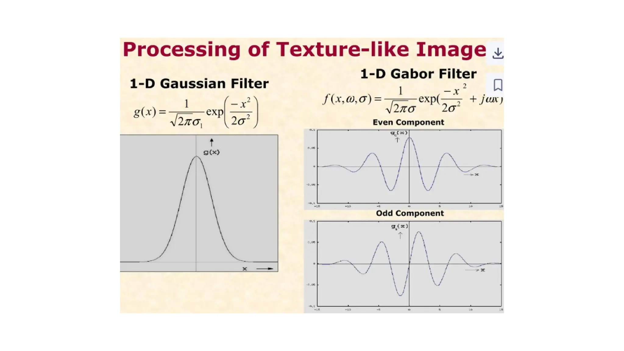
Transform-based methods(Gabor filters)
•Transform-based methods, such as Gabor filters, are a powerful
technique for texture analysis.
• They work by analyzing an image in both the spatial and frequency
domains simultaneously.
• The core idea is to break down a complex image texture into its
constituent frequencies and orientations.
85.
• How GaborFilters Work
• A Gabor filter is a linear filter whose impulse response is a sinusoidal
wave (the carrier) multiplied by a Gaussian function (the envelope). This
structure gives the filter its unique properties:
• Sinusoidal Wave: This component allows the filter to be tuned to a
specific frequency and orientation, much like how the human visual
system processes information. By adjusting the wavelength and
orientation of the sine wave, you can create a filter that is highly
responsive to textures with a particular pattern and direction.
• Gaussian Envelope: This part localizes the filter in the spatial domain. It
ensures that the filter's response is confined to a small, specific region of
the image, allowing for the analysis of local texture features.
• By combining the two, a Gabor filter can identify what frequency and
orientation of a pattern exists at a particular point in an image.
86.
Using a GaborFilter Bank for Texture Analysis
• Instead of a single filter, texture analysis typically uses a Gabor filter bank. This is a
collection of Gabor filters with different orientations and frequencies. Each filter in
the bank is applied to the input image, producing a new, filtered image.
• Filtering: The original image is convolved with each filter in the bank. For a texture
with fine, horizontal stripes, for example, the filter tuned to a high frequency and a
horizontal orientation will have the strongest response.
• Feature Extraction: The output of each filter is often processed to create a feature
vector for each pixel or region of the image. Common features include the mean
and variance of the filtered images, which provide a quantitative measure of the
texture's characteristics.
• Classification/Segmentation: These feature vectors are then used for tasks like
texture segmentation (dividing an image into regions of different textures) or
classification (identifying what kind of texture is present). The process is similar to
how the human brain distinguishes between different textures like brick, wood, or
grass.