Machine Learning and Statistical Analysis

Jong Youl Choi Computer Science Department (jychoi@cs.indiana.edu)

Social Bookmarking Socialized Tags Bookmarks

Principles of Machine Learning Bayes’ theorem and maximum likelihood Machine Learning Algorithms Clustering analysis Dimension reduction Classification Parallel Computing General parallel computing architecture Parallel algorithms

Definition Algorithms or techniques that enable computer (machine) to “learn” from data. Related with many areas such as data mining, statistics, information theory, etc. Algorithm Types Unsupervised learning Supervised learning Reinforcement learning Topics Models Artificial Neural Network (ANN) Support Vector Machine (SVM) Optimization Expectation-Maximization (EM) Deterministic Annealing (DA)

Posterior probability of  i , given X  i 2  : Parameter X : Observations P (  i ) : Prior (or marginal) probability P ( X |  i ) : likelihood Maximum Likelihood (ML) Used to find the most plausible  i 2  , given X Computing maximum likelihood (ML) or log-likelihood  Optimization problem

Problem Estimate hidden parameters (  ={  ,  }) from the given data extracted from k Gaussian distributions Gaussian distribution Maximum Likelihood With Gaussian (P = N ), Solve either brute-force or numeric method (Mitchell , 1997)

Problems in ML estimation Observation X is often not complete Latent (hidden) variable Z exists Hard to explore whole parameter space Expectation-Maximization algorithm Object : To find ML, over latent distribution P ( Z | X ,  ) Steps 0. Init – Choose a random  old 1. E-step – Expectation P ( Z | X ,  old ) 2. M-step – Find  new which maximize likelihood. 3. Go to step 1 after updating  old Ã  new

Definition Grouping unlabeled data into clusters, for the purpose of inference of hidden structures or information Dissimilarity measurement Distance : Euclidean(L 2 ), Manhattan(L 1 ), … Angle : Inner product, … Non-metric : Rank, Intensity, … Types of Clustering Hierarchical Agglomerative or divisive Partitioning K-means, VQ, MDS, … (Matlab helppage)

Find K partitions with the total intra-cluster variance minimized Iterative method Initialization : Randomized y i Assignment of x ( y i fixed) Update of y i ( x fixed) Problem?  Trap in local minima (MacKay, 2003)

Deterministically avoid local minima No stochastic process (random walk) Tracing the global solution by changing level of randomness Statistical Mechanics Gibbs distribution Helmholtz free energy F = D – TS Average Energy D = <  E x > Entropy S = - P (E x ) ln P (E x ) F = – T ln Z In DA, we make F minimized (Maxima and Minima, Wikipedia)

Analogy to physical annealing process Control energy (randomness) by temperature (high  low) Starting with high temperature (T = 1 ) Soft (or fuzzy) association probability Smooth cost function with one global minimum Lowering the temperature (T ! 0) Hard association Revealing full complexity, clusters are emerged Minimization of F, using E( x , y j ) = || x - y j || 2 Iteratively,

Definition Process to transform high-dimensional data into low-dimensional ones for improving accuracy, understanding, or removing noises. Curse of dimensionality Complexity grows exponentially in volume by adding extra dimensions Types Feature selection : Choose representatives (e.g., filter,…) Feature extraction : Map to lower dim. (e.g., PCA, MDS, … ) (Koppen, 2000)

Finding a map of principle components (PCs) of data into an orthogonal space, such that y = W x where W 2 R d £ h (h À d) PCs – Variables with the largest variances Orthogonality Linearity – Optimal least mean-square error Limitations? Strict linearity specific distribution Large variance assumption x 1 x 2 PC 1 PC 2

Like PCA, reduction of dimension by y = R x where R is a random matrix with i.i.d columns and R 2 R d £ p (p À d) Johnson-Lindenstrauss lemma When projecting to a randomly selected subspace, the distance are approximately preserved Generating R Hard to obtain orthogonalized R Gaussian R Simple approach choose r ij = {+3 1/2 ,0,-3 1/2 } with probability 1/6, 4/6, 1/6 respectively

Dimension reduction preserving distance proximities observed in original data set Loss functions Inner product Distance Squared distance Classical MDS: minimizing STRAIN, given  From  , find inner product matrix B (Double centering) From B, recover the coordinates X’ (i.e., B=X’X’ T )

SMACOF : minimizing STRESS Majorization – for complex f(x), find auxiliary simple g(x,y) s.t.: Majorization for STRESS Minimize tr(X T B(Y) Y), known as Guttman transform (Cox, 2001)

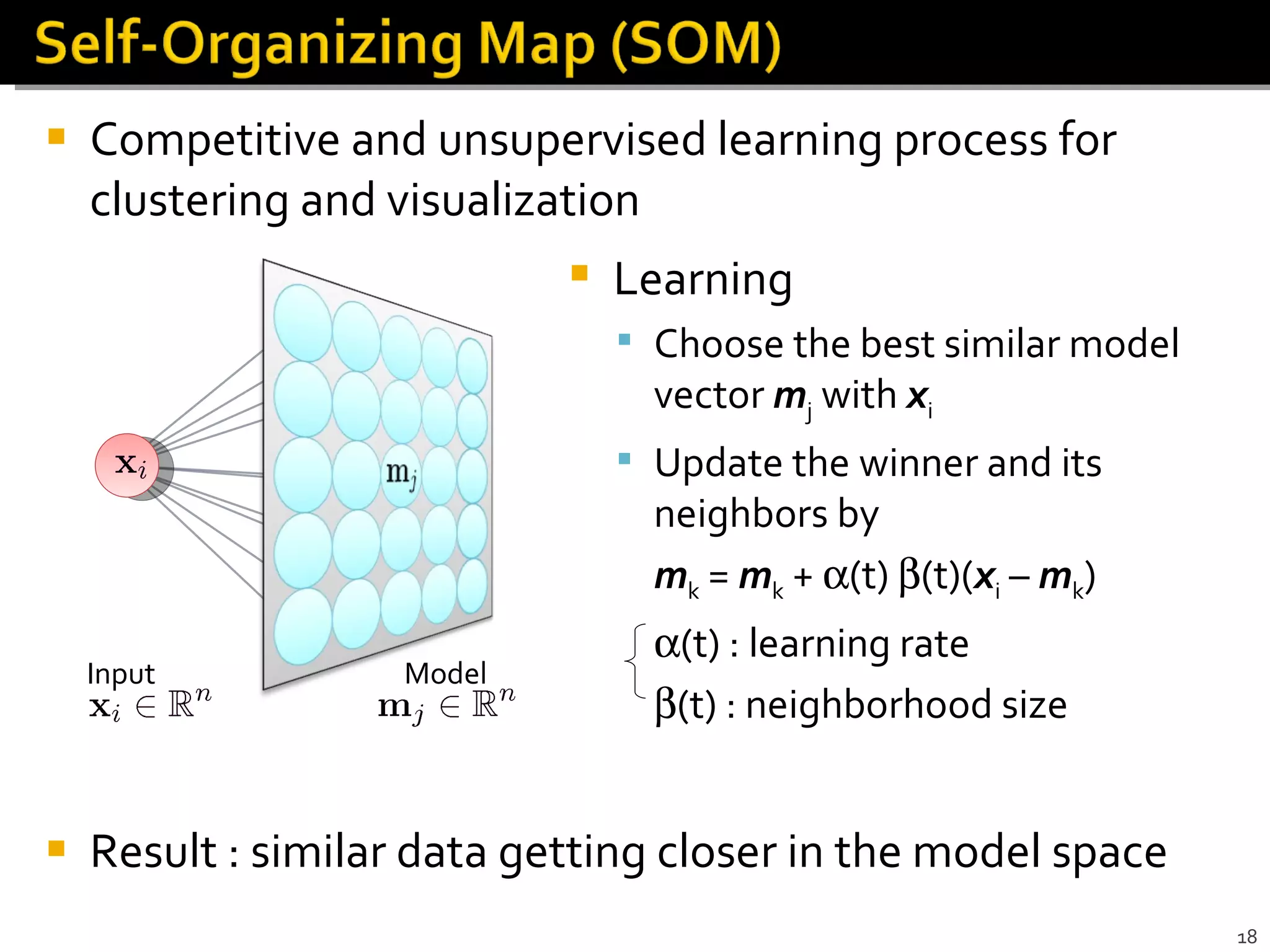
Competitive and unsupervised learning process for clustering and visualization Result : similar data getting closer in the model space Input Model Learning Choose the best similar model vector m j with x i Update the winner and its neighbors by m k = m k +  (t)  (t)( x i – m k )  (t) : learning rate  (t) : neighborhood size

Definition A procedure dividing data into the given set of categories based on the training set in a supervised way Generalization Vs. Specification Hard to achieve both Avoid overfitting(overtraining) Early stopping Holdout validation K-fold cross validation Leave-one-out cross-validation (Overfitting, Wikipedia) Validation Error Training Error Underfitting Overfitting

Perceptron : A computational unit with binary threshold Abilities Linear separable decision surface Represent boolean functions (AND, OR, NO) Network (Multilayer) of perceptrons  Various network architectures and capabilities Weighted Sum Activation Function (Jain, 1996)

Learning weights – random initialization and updating Error-correction training rules Difference between training data and output: E(t,o) Gradient descent (Batch learning) With E =  E i , Stochastic approach (On-line learning) Update gradient for each result Various error functions Adding weight regularization term (  w i 2 ) to avoid overfitting Adding momentum (  w i (n-1) ) to expedite convergence

Q: How to draw the optimal linear separating hyperplane?  A: Maximizing margin Margin maximization The distance between H +1 and H -1 : Thus, || w || should be minimized Margin

Constraint optimization problem Given training set { x i , y i } (y i 2 {+1, -1}): Minimize : Lagrangian equation with saddle points Minimized w.r.t the primal variable w and b: Maximized w.r.t the dual variables  i (all  i ¸ 0) x i with  i > 0 (not  i = 0) is called support vector (SV)

Soft Margin (Non-separable case) Slack variables  i < C Optimization with additional constraint Non-linear SVM Map non-linear input to feature space Kernel function k( x , y ) = h  ( x ),  ( y ) i Kernel classifier with support vectors s i Input Space Feature Space

Memory Architecture Decomposition Strategy Task – E.g., Word, IE, … Data – scientific problem Pipelining – Task + Data Symmetric Multiprocessor (SMP) OpenMP, POSIX, pthread, MPI Easy to manage but expensive Commodity, off-the-shelf processors MPI Cost effective but hard to maintain (Barney, 2007) (Barney, 2007) Shared Memory Distributed Memory

Shrinking Recall : Only support vectors (  i >0) are used in SVM optimization Predict if data is either SV or non-SV Remove non-SVs from problem space Parallel SVM Partition the problem Merge data hierarchically Each unit finds support vectors Loop until converge (Graf, 2005)

Machine Learning and Statistical Analysis

Machine Learning and Statistical Analysis

More Related Content

What's hot

Viewers also liked

Similar to Machine Learning and Statistical Analysis

More from butest

Machine Learning and Statistical Analysis

Editor's Notes