


More Related Content


Similar to Multilayer & Back propagation algorithm (20)


Multilayer & Back propagation algorithm
- 1. SWAPNA.C Asst.Prof. IT Dept. SriDevi Women’s Engineering College
- 2. Multilayer Networks Multilayer networks using gradient descent algorithm. In Perceptron its discontinuous threshold makes it undifferentiable and hence unsuitable for gradient descent. swapna.c
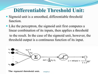
- 3. Differentiable Threshold Unit: Sigmoid unit is a smoothed, differentiable threshold function. Like the perceptron, the sigmoid unit first computes a linear combination of its inputs, then applies a threshold to the result. In the case of the sigmoid unit, however, the threshold output is a continuous function of its input. swapna.c
- 4. More precisely, the sigmoid unit computes its output o as Where is often called the sigmoid function or, alternatively, the logistic function. Its output ranges between 0 and 1, increasing monotonically with its input. It maps a very large input domain to a small range of outputs, it is often referred to as the squashing function of the unit. The sigmoid function has the useful property that its derivative is easily expressed in terms of its output. The function tanh is also sometimes used in place of the sigmoid function swapna.c
- 5. The BACKPROPAGATION ALGORITHM: The BACKPROPAGATION Algorithm learns the weights for a multilayer network, given a network with a fixed set of units and interconnections. It employs gradient descent to attempt to minimize the squared error between the network output values and the target values for these outputs. we are considering networks with multiple output units rather than single units as before, we begin by redefining E to sum the errors over all of the network output units. swapna.c
- 6. where outputs is the set of output units in the network, and tkd and okd are the target and output values associated with the kth output unit and training example d. One major difference in the case of multilayer networks is that the error surface can have multiple local minima, in contrast to the single-minimum parabolic error surface. This is the incremental, or stochastic gradient descent version of BACKPROPAGATION. swapna.c
- 7. swapna.c
- 8. swapna.c
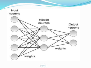
- 9. The algorithm applies to layered feedforward networks containing 2 layers of sigmoid units, with units at each layer connected to all units from the preceding layer. BACK-PROPAGATION. Notations: swapna.c
- 10. Constructing a network with the desired number of hidden and output units and initializing all network weights to small random values. Given this fixed network structure, the main loop of the algorithm then repeatedly iterates over the training examples. calculates the error of the network output for this example, computes the gradient with respect to the error on this example, then updates all weights in the network. This gradient descent step is iterated until the network performs acceptably well. swapna.c
- 11. The gradient descent weight-update rule is similar to the delta training rule. Like the delta rule, it updates each weight in proportion to the learning rate , the input value xji to which the weight is applied, and the error in the output of the unit. The only difference is that the error (t - o) in the delta rule is replaced by a more complex error term. The weight-update loop in BACKPROPAGATION Algorithm be iterated thousands of times in a typical application. swapna.c
- 12. Derivation of the BACKPROPAGATION Rule Recall that stochastic gradient descent involves iterating through the training examples one at a time, for each training example d descending the gradient of the error Ed with respect to this single example. In other words, for each training example d every weight wji is updated by adding to it where Ed is the error on training example d, summed over all output units in the network. Here outputs is the set of output units in the network, tk is the target value of unit k for training example d, and ok is the output of unit k given training example d. swapna.c
- 13. The derivation of the stochastic gradient descent rule is conceptually straightforward, but requires keeping track of a number of subscripts and variables. We will follow the notation adding a subscript j to denote to the jth unit of the network as follows: We can use the chain rule to write swapna.c
- 14. swapna.c
- 15. We consider two cases in turn: the case where unit j is an output unit for the network, and the case where j is an internal unit. Case 1: Training Rule for Output Unit Weights. Just as wji can influence the rest of the network only through net,, net, can influence the network only through oj. Therefore, we can invoke the chain rule again to write swapna.c
- 16. swapna.c
- 17. We have the stochastic gradient descent rule for output units swapna.c
- 18. Case 2: Training Rule for Hidden Unit Weights. In the case where j is an internal, or hidden unit in the network, the derivation of the training rule for wji must take into account the indirect ways in which wji can influence the network outputs and hence Ed. Notice that netj can influence the network output only through the units in Downstream(j). swapna.c
- 19. swapna.c
- 20. A variety of termination conditions can be used to halt the procedure: One may choose to halt after a fixed number of iterations through the loop, or once the error on the training examples falls below some threshold, or once the error on a separate validation set of examples meets some criterion. The choice of termination criterion is an important one, because too few iterations can fail to reduce error sufficiently, and too many can lead to overfitting the training data. swapna.c
- 21. ADDING MOMENTUM In the algorithm by making the weight update on the nth iteration depend partially on the update that occurred during the (n - 1)th iteration, as follows: is the weight update performed during the nth iteration through the main loop of the algorithm, and 0 < < 1 is a constant called the momentum. The 1st term in the right equation is weight-update rule and 2nd term momentum term. swapna.c
- 22. The effect of is to add momentum that tends to keep the ball rolling in the same direction from one iteration to the next. This can sometimes have the effect of keeping the ball rolling through small local minima in the error surface, or along flat regions in the surface where the ball would stop if there were no momentum. It also has the effect of gradually increasing the step size of the search in regions where the gradient is unchanging, thereby speeding convergence. swapna.c
- 23. LEARNING IN ARBITRARY ACYCLIC NETWORKS The definition of BACKPROPAGATION applies only to two-layer networks. In general, the value for a unit r in layer m is computed from the values at the next deeper layer m+1 according to We really saying here is that this step may be repeated for any number of hidden layers in the network. swapna.c
- 24. It is equally straightforward to generalize the algorithm to any directed acyclic graph, regardless of whether the network units are arranged in uniform layers as we have assumed up to now. In the case that they are not, the rule for calculating for any internal unit is Where Downstream(r) is the set of units immediately downstream from unit r in the network: that is, all units whose inputs include the output of unit r. swapna.c
- 25. REMARKS ON THE BACKPROPAGATION ALGORITHM Convergence and Local Minima: BACKPROPAGATION over multilayer networks is only guaranteed to converge toward some local minimum in E and not necessarily to the global minimum error. When gradient descent falls into a local minimum with respect to one of these weights, it will not necessarily be in a local minimum with respect to the other weights. A second perspective on local minima can be gained by considering the manner in which network weights evolve as the number of training iterations increases. swapna.c
- 26. Common heuristics to attempt to alleviate the problem of local minima include: Add a momentum term to the weight-update rule. Momentum can sometimes carry the gradient descent procedure through narrow local minima. Use stochastic gradient descent rather than true gradient descent. Train multiple networks using the same data, but initializing each network with different random weights. If the different training efforts lead to different local minima, then the network with the best performance over a separate validation data set can be selected. swapna.c
- 27. Representational Power of FeedForward Networks 3 general rules of FeedForward network. Boolean functions. Every Boolean function can be represented exactly by some network with two layers of units, although the number of hidden units required grows exponentially in the worst case with the number of network inputs. Continuous functions. Every bounded continuous function can be approximated with arbitrarily small error (under a finite norm) by a network with two layers of units swapna.c
- 28. Arbitrary functions. Any function can be approximated to arbitrary accuracy by a network with three layers of units (Cybenko 1988). Again, the output layer uses linear units, the two hidden layers use sigmoid units, and the number of units required at each layer is not known in general. The proof of this involves showing that any function can be approximated by a linear combination of many localized functions that have value 0 everywhere except for some small region, and then showing that two layers of sigmoid units are sufficient to produce good local approximations. swapna.c
- 29. Hypothesis Space Search and Inductive Bias hypothesis space is the n-dimensional Euclidean space of the n network weights. This hypothesis space is continuous, in contrast to the hypothesis spaces of decision tree learning and other methods based on discrete representations. Inductive Bias is depends on the interplay between the gradient descent search and the way in which the weight space spans the space of represent able functions. However, one can roughly characterize it as smooth interpolation between data points. swapna.c
- 30. Hidden Layer Representations One intriguing property of BACKPROPAGATION its ability to discover useful intermediate representations at the hidden unit layers inside the network. swapna.c
- 31. Generalization, Overfitting, and Stopping Criterion BACKPROPAGATION is susceptible to overfitting the training examples at the cost of decreasing generalization accuracy over other unseen examples. BACKPROPAGATION will often be able to create overly complex decision surfaces that fit noise in the training data or unrepresentative characteristics of the particular training sample. Several techniques are available to address the overfitting problem for BACKPROPAGATION learning. One approach, known as weight decay, is to decrease each weight by some small factor during each iteration. swapna.c
- 32. One of the most successful methods for overcoming the overfitting problem is to simply provide a set of validation data to the algorithm in addition to the training data. The algorithm monitors the error with respect to this validation set, while using the training set to drive the gradient descent search. The problem of overfitting is most severe for small training sets. swapna.c
- 33. In these cases, a k-fold cross-validation approach is sometimes used, in which cross validation is performed k different times, each time using a different partitioning of the data into training and validation sets, and the results are then averaged. In one version of this approach, them available examples are partitioned into k disjoint subsets, each of size m/k. The cross validation procedure is then run k times, each time using a different one of these subsets as the validation set and combining the other subsets for the training set. swapna.c