Create Dynamic Chart Between Two Dates in Excel

Excel is a powerful tool that enables users to analyze and present data in a variety of ways. One useful feature of Excel is the ability to create dynamic charts that update automatically based on the user's inputs. In this tutorial, we will explore how to create a dynamic chart between two dates in Excel using date ranges as the criteria for selecting the data to display. By the end of this tutorial, you will be able to create a chart that shows a range of data based on the dates you choose, making it easier to visualize trends and patterns in your data. Whether you are a business professional, a student, or just someone who wants to learn more about Excel, this tutorial will provide you with the tools you need to create a dynamic chart that meets your specific needs.

Create A Dynamic Chart Between Two Dates (Based On Dates

Here we will first copy the column then remove the duplicates then finally create the chart. So let us see a simple process to know how you can create a dynamic chart between two dates (based on dates) in excel.

Step 1

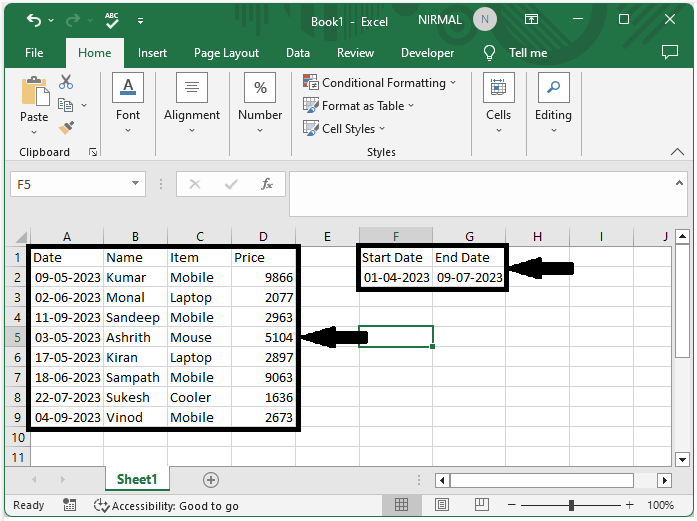
Consider an Excel sheet where the data is similar to the below image.

First, copy the item column to another range as shown in the below image

Step 2

Then select the range of cells and click on "Data," then click "Remove Duplicates" and click OK.

Select cells > Data > Remove Duplicates > Ok.

Step 3

Now click on an empty cell in our case cell J2 and enter the formula as =SUMIFS($D$2:$D$9,$C$2:$C$9,I2,$A$2:$A$9,">="&$F$2,$A$2:$A$9,"<="&$G$2) and click enter to get the first value.

Empty cell > Formula > Enter.

Step 4

Then drag down from the first value to fill all the results.

Step 5

Now finally select the range of cells, click on insert, and select any chart to complete our task

Select cell > Insert > Chart.

Conclusion

In this tutorial, we have used a simple example to demonstrate how you can create a dynamic chart between two dates (based on dates) in Excel to highlight a particular set of data.